Prerequisite Topics

Elliptic Curve Pairings

$\mathcal{P} \mathfrak{lon}\mathcal{K}$ also uses Elliptic Curve Pairings. If you aren’t familiar with Pairings, here is an introduction to Elliptic Curve Pairings. The MOV attack itself is not relevant to the current post. The same link also contains a brief description of the roots of unity in a finite field which are relevant.

Polynomial Commitment Schemes

$\mathcal{P} \mathfrak{lon}\mathcal{K}$ uses a polynomial commitment scheme like KZG. You can read about the KZG Polynomial Commitment Scheme here. This link also covers the additional additional batch processing protocols not present in the KZG paper but used in $\mathcal{P} \mathfrak{lon}\mathcal{K}$.

The Schwartz-Zippel Lemma

Let $f$ be a polynomial from $\mathbb F_p[x]$ of degree less than or equal to $d$. Let $p \approx 2^{256}$ & $d \le 2^{40}$. If we test $f$ at a random value $r \in \mathbb F_p$, then the probability that $f(r) = 0$ would be $\frac {d}{p}$ which for these values of $d$ & $p$ would be very, very small. So, if $f(r) = 0$, then with high probability, $f$ is a zero polynomial (i.e., zero at all points). This is a simple test to check if a committed polynomial is a zero polynomial. Open the commitment to the polynomial at a random point & if it opens to zero, then it is a zero polynomial.

This also helps to prove that 2 polynomials are equal. If the 2 polynomials are $f$ & $g$, we create a new polynomial $p(x) = f(x)\space - \space g(x)$.

If we test $p$ at a random $r \in \mathbb F_p$ & $f(r)$ turns out to be $0$, then $p$ is a zero polynomial with very high probability. If $p$ is a zero polynomial, then it obviously means $f = g$

Note: The target audience for this post is someone with a basic knowledge of zkSNARKs in general without knowing much about $\mathcal{P} \mathfrak{lon}\mathcal{K}$. Here is a post about an older SNARK - Groth16.

The example

$\mathcal{P} \mathfrak{lon}\mathcal{K}$ operates in a field $\mathbb F_p$.

Consider the equation

$x^3 + x + 5 = 73$

We use this equation in our toy example & we use a multiplicative subgroup of $\mathbb F_{97}$

The Prover knows a witness which satisfies this equation & wants to prove to the Verifier that she knows it.

This is the Circuit and its trace for the witness ($x=4$)

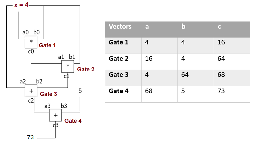
This circuit will be expressed using Gate Constraints and Copy Constraints.

Gate Constraints

This is the Gate Constraint Equation

${q_L}_i\cdot a_i + {q_R}_i\cdot b_i + {q_M}_i\cdot (a_i\cdot b_i) + {q_C}_i + {q_O}_i\cdot c_i = 0$

Here $i$ takes values from the set $[n] = \lbrace1, 2, 3, …, n\rbrace$ - i.e., depending on the gate. The $a$s & the $b$s represent the left & right input of the $i$th gate & the $c$s represents the corresponding output.

The $q$’s are known as the selectors. For an addition gate, $q_L$ & $q_R$ will be set to $1$ while $q_M$ will be set to $0$. $q_C$ represents the constant if any in the equation

Likewise for a multiplication gate, $q_L$ & $q_R$ will be set to $0$ while $q_M$ will be set to $1$

Gate 1:

Gate 1 is a multiplication Gate representing

$4 \times 4 = 16$

The Gate Constraint values for this would be

$0\cdot 4 + 0\cdot 4 + 1 \cdot (4\cdot 4) + 0 + (-1)\cdot 16 = 0$

Gate 2

$16 \times 4 = 64$

$0\cdot 16 + 0\cdot 4 + 1 \cdot (16\cdot 4) + 0 + (-1)\cdot 64 = 0$

Gate 3

Gate 3 is an addition gate representing

$64 + 4 = 68$

$1.64+1.4 + 0\cdot (64\cdot4) + 0 + (-1)\cdot 68 = 0$

Gate 4

$68 + 5 - 73 = 0$

$1.68+ 0.0 + 0\cdot (68\cdot0) + 5 + (-1)\cdot 73 = 0$

We can collect all $q$s, $a$s, $b$s & $c$s into vectors.

$q_L = [0, 0, 1, 1]$

$q_R = [0, 0, 1, 0]$

$q_M = [1, 1, 0, 0]$

$q_C = [0, 0, 0, 5]$

$q_O = [-1, -1, -1, -1]$

$a = [4, 16, 4, 68]$

$b = [4, 4, 64, 0]$

$c = [16, 64, 68, 73]$

We need to check that the output of each Gate is calculated correctly.

We now interpolate each of these vectors to create a polynomial representation of that vector. For reasons explained here, $\mathcal{P} \mathfrak{lon}\mathcal{K}$ uses a multiplicative subgroup to represent the gates. In this example, we have 4 gates & so we need a multiplicative subgroup of order 4 formed by a 4th root of unity. We can use the multiplicative subgroup generated by the 4th root of unity $\omega = 22$ i.e., $H = \lbrace 1, \omega, \omega^2, \omega^3 \rbrace$ - $1$ represents Gate 1, $\omega$ represents Gate 2 & so on & so forth.

Let’s interpolate $a = [4, 16, 4, 68]$. We interpolate this as the points $[(1,4), (\omega,16), (\omega^2,4), (\omega^3,68)]$

In sagemath

sage: F97 = GF(97)
sage: R97.<x> = PolynomialRing(F97)
sage: ω = F97(4)
sage: pts = [(ω^0,4), (ω,16), (ω^2,4), (ω^3,68)]
sage: R97.lagrange_polynomial(pts)
68*x^3 + 59*x^2 + 27*x + 44

(Note: The ω used here is omega, the 4th root of unity, and not ‘w’ which is the witness).

That gives us $a(X)$.

Interpolating for other vectors also, we get,

$a(X) = 68x^3 + 59x^2 + 27x + 44$

$b(X) = 95x^3 + 10x^2 + 89x + 4$

$c(X) = 58x^3 + x^2 + 54x$

This is done in Round 1

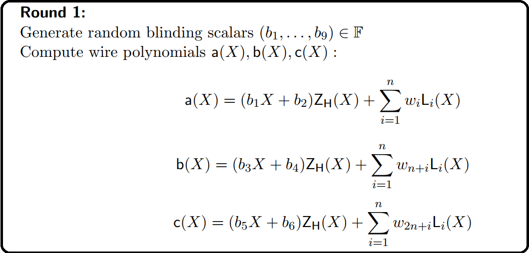
The term $(b_i X + b_{i+1})z_H(X)$ is added to each for blinding which is explained here

The selector polynomials are also computed by interpolation from the selector vectors.

$q_L(X) = 19x^3 + 79x^2 + 79x + 17$

$q_R(X) = 19x^3 + 79x^2 + 79x + 17$

$q_M(X) = 78x^3 + 18x^2 + 18x + 81$

$q_C(X) = 68x^3 + 27x^2 + 86x + 13$

$q_O(X) = 96$

(Note: There is also a Public Input Polynomial which is created using Public Variables. The difference between a Public Input & a constant is that the public variable can change every time while constant remains the same for the circuit. Because of this $q_C$ can be preprocessed & reused for the circuit. Pre-processing means it is part of the one-time initial set up computation of the system before the generation of any proofs. The $\mathcal{P} \mathfrak{lon}\mathcal{K}$ paper has the Public Input Polynomial $PI(X)$ - I am ignoring it here because it’s treated very similar to $q_C$ except that it can be preprocessed.)

Using our Gate Constraint Equation, we get the Gate Constraint Polynomial as

$g(X) = a(X)b(X)q_M(X) + a(X)q_L(X) + b(X)q_R(X) + c(X)q_O(X) + qC(X)$

We use this to prove that Gate Constraints are satisfied. While interpolating all these individual polynomials, we used elements of $H$ as the x-coordinate. So, proving that $g(X) = 0$ on all elements of $H$ would prove the Gate Constraints.

If a polynomial is $0$ on all elements of $H$, it would mean that each element of $H$ is a root of the polynomial - i.e., the polynomial is exactly divisible by the vanishing polynomial $z_H(X) = (X-1)(X-\omega)(X-\omega^2)…(X-\omega^{n-1})$

As explained here, this is the same as

$z_H(X) = X^n - 1$

So, the prover can compute $t(X)= \frac {g(X)}{z_H(X)}$ & provide a commitment to $t(X)$ & the opening proof. The prover would be able to do it only $t(X)$ is $0$ on every element of $H$ which will ensure that $g(X)$ is exactly divisible by $z_H(X)$ and that would prove the Gate Constraints.

This is done in Round 3.

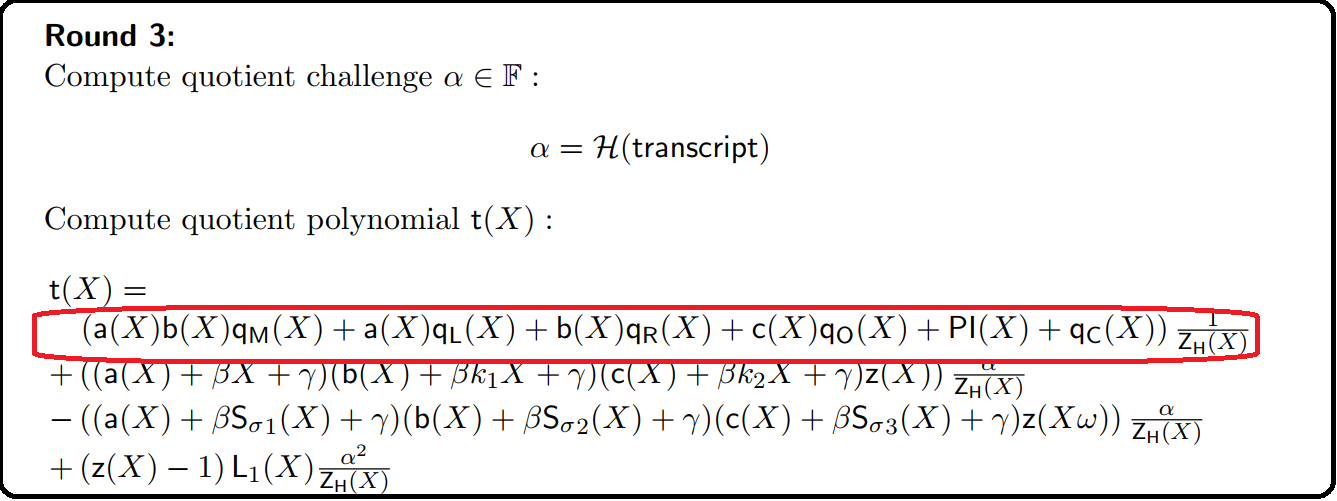
Instead proving multiple different polynomials (3 different polynomials are added together to form $t(X)$ above) are zero at $H$, $\mathcal{P} \mathfrak{lon}\mathcal{K}$ combines them as linearly independent terms so that proving $t(X) = 0$ proves that each of those 3 polynomials are 0 on $H$. That’s why you see the $\alpha$ terms as explained here.

Copy Constraints

$\mathcal{P} \mathfrak{lon}\mathcal{K}$ also checks the Copy constraints as explained here in a separate post on the $\mathcal{P} \mathfrak{lon}\mathcal{K}$ Permutation Check.

Remaining Rounds

The Permutation Polynomial contains multiplication of three polynomials of degree $n-1$. So, this will result in a polynomial of degree close to $3n$. Round 3 splits the quotient polynomial $t(X)$ into multiple parts as explained here.

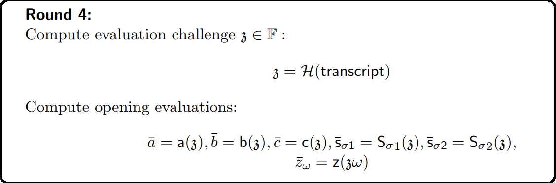
Round 4 above is preparation for the Field Element Reduction Optimisation. The prover computes evaluation of a few polynomials which form the quotient polynomial of Round 3 & sends commitments & opening proofs for them to the verifier.

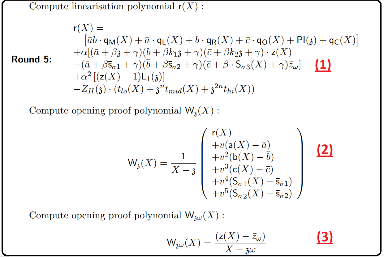
The 3 parts of the above screenshot

$(1)$ Round 5 creates the Linearisation Polynomial $r(X)$ using the evaluations sent in Round 4. If you notice, as discussed in the Field Element Optimisation, wherever polynomials in $t(X)$ were multiplied with other polynomials, there one or more of those polynomials are substituted by the evaluation at $\mathfrak{z}$ in $r(X)$ so that the commitments to the remaining polynomials can be added up by the verifier to compute the commitment for $r(X)$ without the prover needing to send him the commitment.

For e.g., the term $a(X)b(X)q_M(X)$ at the beginning of $t(X)$ (in Round 3) - this is a multiplication of 3 polynomials. In round 4, evaluations of $a$ and $b$ at $X = \mathfrak{z}$ were sent to the verifier - i.e., $\bar a = a(\mathfrak{z})$ and $\bar b = b(\mathfrak{z})$.

In the above screenshot, the term $a(X)b(X)q_M(X)$ in $t(X)$ becomes $\bar a\bar b\cdot q_M(X)$ in $r(x)$ so that the commitment for $\bar a\bar b\cdot q_M(X)$ can be computed by multiplying the commitment for $q_M(X)$ by the product of the values $\bar a$ & $\bar b$. In Round 4, prover also sends $\bar c = c(\mathfrak{z}),\bar s_{\sigma_1} = S_{\sigma_1}(\mathfrak{z}),\bar s_{\sigma_2} = S_{\sigma_2} = (\mathfrak{z}),\bar {z\omega} = z(\mathfrak{z}\omega)$ so that the commitment to $r(X)$ can be computed by the verifier.

$(2)$ The verifier needs to verify that $r(X)=0$ (which will verify that the other polynomials which are combined to form $r(X)$ are $0$ at all elements of $H$. The verifier also needs to verify the evaluations of $a(X), b(X), c(X), S_{\sigma_1}(X)$ & $S_{\sigma_2}(X)$ sent by the prover are correct.

The prover combines $r(X)$ with all these in a linearly independent way using $\lbrace 1, v, v^2, v^3, v^4, v^5 \rbrace$. Since these are all evaluated at $\mathfrak{z}$, we divide the combination with $(1-\mathfrak{z})$ (why is explained in the KZG post). This creates the opening proof polynomial $W_{\mathfrak{z}}(X)$

$(3)$ If you check $t(X)$, it has both $z(X)$ & $z(X\omega)$ terms. We already have a commitment to $z$ from Round 2. We compute the opening proof polynomial $W_{\mathfrak{z}\omega}(X)$ for $z(X)$ at $\mathfrak{z}\omega$.

This ends the prover steps.

The verifier verifies using KZG batched protocol.