The Prover wants to prove to the Verifier that she knows the solution to a particular equation without revealing the solution itself. In order for her to to do this, in the Pinnochio & Groth16 zkSNARKs, she has to first transform the equation into the QAP (Quadratic Arithmetic Program) form. This post explains only the conversion part of these zkSNARKs.

This post is based on Vitalik Buterin’s write up on the same topic (with a partially similar title) but with some changes.

• In his write up, he doesn’t operate in a finite field though in the real world all these operations are done in a finite field. I think he has avoided finite fields to simplify the write up. However, I think not using finite fields ends up complicating it instead of simplifying it. His examples end up with scary looking floating point numbers. Working a finite field avoids this. Also since floating point operations are not precise, so his final $T/Z$ polynomial division which should have no remainder ends up with an infinitesimal remainder if you try it out yourself.

• In the R1CS to QAP part of the transformation & beyond, I have shown the implementation using sagemath.

The equation

$x^3 + x + 5 = 35$ is the cubic equation the Prover knows the solution to & she has to convince the Verifier about this without revealing the solution to him. The solution is $x=3$

If you were to write a program in Python which takes a value for $x$ & evaluates the computation part of this equation, it would look something like this

def Evaluate(x):
    return x**3 + x + 5

Code Flattening

We first decompose the above code into a series of much simpler operations. This step is called flattening. In the flattened code, we are allowed only the following operations

• Assignment i.e. $x = y$, where $x$ is be a variable and $y$ can be a variable or a constant
• Operations like $x = y$ (Operator) $z$, where $x$ is a variable and $y$ and $z$ can be variables or constants. The only operators allowed are $+, -, *, /$

There is no return statement in the flattened code. Instead, we assign the return value to a variable “out”.

The flattened code

def Evaluate(x):
    var1 = x * x 
    var2 = var1 * x 
    var3 = var2 + x
    out  = var3 + 5

Conversion to Arithemetic Circuits & then R1CS

Next, we draw an arithmetic circuit of the above flattened program.

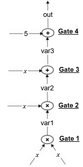
As we see from the circuit diagram, the circuit has 4 gates representing multiplication & addition operations & also has 5 variables & a constant $5$.

Let’s represent the variables in a solution vector $S$ (also called as witness)

$S = [1, x, out, var1, var2, var3]$

$1$ is included as an element of the vector so as to represent constants. For e.g. if we need a constant $5$, it will be represented as $5 * 1$

We now convert the Arithmetic Circuit into a Rank-1 Constraint System (R1CS). A R1CS is a triplet of vectors $(l, r, o)$, and a solution vector $S$, such that $(l\cdot S) * (r\cdot S) = (o\cdot S)$ where $(\cdot)$ is the dot-product. Here $l$ stands for left (or left hand side of the multiplication) & $r$ for right of the multiplication & $o$ for output of each gate. We will have one triplet/constraint for each of the arithmetic gates.

Gate 1

Now in the circuit diagram, let’s take the first gate which represents $var1 = x * x$

For the purpose of the conversion, we look at it as $x * x = var1$. We now represent it as 3 vectors $l, r, o$. $l$ & $r$ is the vector on the left & right of the gate & $o$ is the output vector.

$l = [0, 1, 0, 0, 0, 0]$ (This represents the term $x$ which is to the left of the multiplication gate. Every element of the $l$ vector is 0 except the element corresponding to $x$ which has the value 1)

$r = [0, 1, 0, 0, 0, 0]$ (This represents the term $x$ which is to the right of the multiplication gate. Every element of the $r$ vector is 0 except the element corresponding to $x$ which has the value 1)

$o = [0, 0, 0, 1, 0, 0]$ (This represents $var1$ which is the output of the multiplication gate. Every element of the $o$ vector is 0 except the one corresponding to $var1$ which has the value 1)

Any solution vector which is correct will satify $(l.S) * (r\cdot S) = (o\cdot S)$.

Let us try this out. We know the solution of the equation $x^3 + x + 5 == 35$ is $x = 3$. So substitute our solution vector $S = [1, x, out, var1, var2, var3]$ with the actual values based on $x = 3$

$var1 = x * x = 3 * 3 = 9$

$var2 = var1 * x = 9 * 3 = 27$

$var3 = var2 + x = 27 + 3 = 30$

$out = var3 + 5 = 30 + 5 = 35$

So $S = [1, 3, 35, 9, 27, 30]$

Dot product of any two vectors $p = [p_1, p_2, …, p_n]$ and $q = [q_1, q_2, …, q_n]$ is defined as

$p \cdot q = \sum_{i=1}^{n} = {p_1}{q_1} + {p_2}{q_2} + … + {p_n}{q_n}$

So $l\cdot S = [0, 1, 0, 0, 0, 0]\cdot[1, 3, 35, 9, 27, 30]$

$l\cdot S = 0 * 1 + 1 * 3 + 0 * 35 + 0 * 9 + 0 * 27 + 0 * 30 = 3$

Likewise $r.S = 3$ and $o.S = 9$

So $(l\cdot S) * (r\cdot S) = 3 * 3 = 9 = (o\cdot S)$.

So $(l\cdot S) * (r\cdot S) = (o\cdot S)$ is satisfied - this is a satisfied R1CS - it shows that the solution vector satisfies Gate 1

Gate 2

Let’s take the 2nd gate which represents $var1 * x = var2$

$l = [0, 0, 0, 1, 0, 0]$ (This represents the term $var1$ which is to the left of the multiplication gate. Every element of the $l$ vector is 0 except the element corresponding to $var1$ which has the value 1)

$r = [0, 1, 0, 0, 0, 0]$ (This represents the term $x$ which is to the left of the multiplication gate. Every element of the $r$ vector is 0 except the element corresponding to $x$ which has the value 1)

$o = [0, 0, 0, 0, 1, 0]$ (This represents the term $var2$ which is the output of the multiplication gate. Every element of the $o$ vector is 0 except the element corresponding to $var2$ which has the value 1)

Gate 3

3rd gate is the addition gate which represents $var2 + x = var3$. The vectors for addition gates are derived differently. The equation is equivalent to $(var2 + x) * 1 = var3$. So the $l$ vector represents $var2 + x$, the $r$ vector represents $1$ & the $o$ vector represents $var3$

$l = [0, 1, 0, 0, 1, 0]$ (This represents $var2 + x$)

$r = [1, 0, 0, 0, 0, 0]$ (This represents $1$)

$o = [0, 0, 0, 0, 0, 1]$ (This represents $var3$)

Gate 4

Likewise, the 4th gate $var3 + 5 = out$ is equivalent to $(var3 + 5) * 1 = out$

$l = [5, 0, 0, 0, 0, 1]$ ($var3 + 5$)

$r = [1, 0, 0, 0, 0, 0]$ ($1$)

$o = [0, 0, 1, 0, 0, 0]$ ($out$)

Though we aren’t explicitly calculating & showing it here, $(l\cdot S) * (r\cdot S) = (o\cdot S)$ is satisfied for Gates 2, 3 & 4 also. We now have the complete R1CS with 4 constraints.

We can create a Matrix $L$ by using each of $l$ vectors as a row in the Matrix. Likewise Matrices $R$ & $O$.

The Complete Satisfied R1CS is

\(L = \begin{pmatrix} 0&1&0&0&0&0 \\ 0&0&0&1&0&0 \\ 0&1&0&0&1&0 \\ 5&0&0&0&0&1 \end{pmatrix}\) \(R = \begin{pmatrix} 0&1&0&0&0&0 \\ 0&1&0&0&0&0 \\ 1&0&0&0&0&0 \\ 1&0&0&0&0&0 \\ \end{pmatrix}\) \(O = \begin{pmatrix} 0&0&0&1&0&0 \\ 0&0&0&0&1&0 \\ 0&0&0&0&0&1 \\ 0&0&1&0&0&0 \\ \end{pmatrix}\)

This along with our solution vector $S = [1, x, out, var1, var2, var3]$ forms our R1CS.

Let’s define these matrices in sage. As said before, we will work in a finite field, say $GF(41)$. We will define all 3 matrices $L,R,O$ in the field. I have shown only 1 below, but the remaining 2 will also be defined similarly.

sage: F41 = GF(41)
....:
....: L = Matrix(F41,[
....:     [0,1,0,0,0,0],
....:     [0,0,0,1,0,0],
....:     [0,1,0,0,1,0],
....:     [5,0,0,0,0,1]]
....:     )

QAP

The next step is taking this R1CS and converting it into the QAP form, which implements the exact same logic except using polynomials. In the construction used, the number of polynomials & their degree would depend on the length of the solution vector & the number of gates. The solution vector contains 6 elements, so we can construct 6 polynomials. Each gate contributes 1 point to each polynomial. We have 4 gates here, we get 4 points per polynomial. 4 points allows us to define a polynomial of maximum degree 3. So we can contruct 6 polynomials each with a maximum degree of 3. So we can transform our matrices collectively into 6 polynomials, each of degree 3.

A polynomial of degree $n$ is defined by a minimum of $n+1$ points. Each column of $L$, $R$ & $O$ has 4 elements. So each such column can be converted into a polynomial of degree 3. We use Lagrange’s Polynomial Interpolation to do this.

For e.g. 1st column of $L$ is $[0, 0, 0, 5]^T$ (shown transposed). We can consider each element as the y-coordinate corresponding to $x \in [1, 2, 3, 4]$. So we get 4 sets of points - $(1,0), (2,0), (3,0), (4,5)$. This is an arbitrary interpretion which we use to convert the R1CS into the QAP form.

We can find the polynomial passing through these 4 points using Lagrange Interpolation.

sage: R41.<x> = PolynomialRing(F41) # Polynomial Ring in GF(41)
....: points = [(1,0), (2,0), (3,0), (4,5)]
....: R41.lagrange_polynomial(points)
....:
35*x^3 + 36*x^2 + 16*x + 36

So the polynomial corresponding to the first Column of $L$ is

$35x^3 + 36x^2 + 16x + 36$

Since we have 18 polynomials to interpolate, we can do it in loops in sage. And after calling R41.lagrange_polynomial(points), we call the coefficients method on the output polynomial (i.e. R41.lagrange_polynomial(points).coefficients(sparse=False)) which transforms the coefficients of each output polynomail into a list which we then collect in a Matrix.

sage: M = [L, R, O]
....: PolyM = []
....:
....: for m in M:
....:     PolyList = []
....:     for i in range(m.ncols()):
....:         points = []
....:         for j in range(m.nrows()):
....:             points.append([j+1,m[j,i]])
....:
....:         Poly = R41.lagrange_polynomial(points).coefficients(sparse=False)
....:
....:         if(len(Poly) < m.nrows()):
....:             # if degree of the polynomial is less than 4
....:             # we add zeroes to represent the missed out terms
....:             dif = m.nrows() - len(Poly)
....:             for c in range(dif):
....:                 Poly.append(0);
....:
....:         PolyList.append(Poly)
....:
....:     PolyM.append(Matrix(F41, PolyList))

If we print out the 3 matrices holding 6 polynomials each we get

# PolyM[0] = Lm (Matrix of L Polynomials) 

[36 16 36 35]
[ 8 16  5 13]
[ 0  0  0  0]
[35 30 37 21]
[ 4 34 24 20]
[40 36 40  7]


# PolyM[1] = Rm (Matrix of R Polynomials)

[ 3 29 23 27]
[39 12 18 14]
[ 0  0  0  0]
[ 0  0  0  0]
[ 0  0  0  0]
[ 0  0  0  0]

# PolyM[2] = Om (Matrix of O Polynomials)

[ 0  0  0  0]
[ 0  0  0  0]
[40 36 40  7]
[ 4 23 22 34]
[35 30 37 21]
[ 4 34 24 20]

For convinience, we will refer to $PolyM[0]$, $PolyM[1]$ & $PolyM[2]$ as $Lm$,$Rm$ & $Om$

You can see the polynomial we got from the first column of $L$ (i.e $35x^3 + 36x^2 + 16x + 36$) appear in first row here of the Matrix $Lm$ . The Row is to be interpreted in reverse order - i.e $[36\ 16\ 36\ 35]$ is $35x^3 + 36x^2 + 16x + 36$

This finishes the transformation of the problem to the QAP Form. What do we achieve by converting it into the QAP form? Instead of checking the constraints in the R1CS individually, we can now check all of the constraints at the same time by doing the dot product check on the polynomials.

Let’s take a closer look at $Lm$

This has 6 left polynomials, one in each row.

Our solution vector $S = [1, x, out, var1, var2, var3]$ also has 6 elements. So we can do a dot product of $S\cdot Lm$ whose output again will be a polynomial. Likewise for the other 2 polynomial matrices.

sage: # We define the solution vector also in the field
....: S = vector(F41,[1, 3, 35, 9, 27, 30])
....: # Create the Lx, Rx & Ox polynomial
....: Lx = R41(list(S*PolyM[0]))
....: Rx = R41(list(S*PolyM[1]))
....: Ox = R41(list(S*PolyM[2]))
....: print("Lx = " + str(Lx))
....: print("Rx = " + str(Rx))
....: print("Ox = " + str(Ox))
Lx = 29*x^3 + 18*x^2 + 36*x + 2
Rx = 28*x^3 + 36*x^2 + 24*x + 38
Ox = 37*x^3 + 37*x^2 + 17*x

So by taking a dot product of $S$ with each of $Lm$, $Rm$ and $Om$, we created 3 polynomials $Lx$, $Rx$ and $Ox$

We can define a new polynomial $T = (S\cdot Lx) * (S\cdot Rx) - (S\cdot Ox)$.

....: # New Polynomial T
....: T = Lx*Rx - Ox
....: print("T(x) = ", end="")
....: print(T)
T(x) = 33*x^6 + 31*x^5 + 15*x^4 + 20*x^3 + 25*x^2 + 5*x + 35

In the R1CS, we had checked if $(l\cdot S) * (r\cdot S) = (o\cdot S)$ for each of the Gates. After conversion to QAP, we can do the same by checking the value of $T$ at $x$ at $1, 2, 3, 4$ - if all 4 are zero, then we have checked all the constraints together - thereby proving that the solution vector known to the Provers satisfies the equation.

....: #Let's check Tx at x = 1, 2, 3, 4
....: print("T(1) = " + str(T(1)))
....: print("T(2) = " + str(T(2)))
....: print("T(3) = " + str(T(3)))
....: print("T(4) = " + str(T(4)))
....:
T(1) = 0
T(2) = 0
T(3) = 0
T(4) = 0

However, the Verifier doesn’t know the polynomial $T$, nor can he compute it since he doesn’t know the solution vector. So the Prover has to prove it to the Verifier that $T$ is zero at $x=1, x=2, x=3,x=4$. If $T$ is zero at $x=1, x=2, x=3,x=4$, then it means these are all roots of $T$. So we create a new polynomial $Z$ known by both the Prover & the Verifier.

$Z = (x-1)(x-2)(x-3)(x-4)$

If $T$ is divided by $Z$, then it will be perfectly divisible & will leave no remainder i.e. there must exist a Polynomial $H$ such that $T(x) = H(x) \cdot Z(x)$

Let’s check this out in sagemath

Z = R41((x-1)*(x-2)*(x-3)*(x-4))
H = T.quo_rem(Z)
print("Quotient of Z/T = ", end="")
print(H[0])
print("Remainder of Z/T = ", end="")
print(H[1])

Quotient of Z/T = 33*x^2 + 33*x + 10
Remainder of Z/T = 0

The reason we get a $0$ remainder is because $Z$ divides $T$. If you change even a single element in the solution vector, then $T$ will no longer divide $Z$ exactly & you will end up with a remainder.

In Groth16, the prover proves that $Z$ exactly divides $T$ using Polynomial Commitments & Elliptic Curve Bilinear Pairings. How it’s done is beyond the scope of this post.

However, you can take a look at my writeup on Commitments & Pairings (without connecting them to Groth16) here

• The KZG/Kate Polynomial Commitment Scheme

• Weil Pairing & the MOV attack writeup introduces Pairings