I have created an updated version of this page - click below to visit the new page

R1CS and QAP (zkSNARKs) : From Zero to Hero with Finite Fields & sagemath.

Peggy wants to prove to Victor that she knows the solution to a particular equation without revealing the solution itself. In order for her to apply zkSNARKs to prove this, she has to first transform this into the QAP(Quadratic Arithmetic Progam) form. This page is a write-up on how to do that. It does not touch upon why we do this & nor does it cover any other parts of zkSNARKs.

Let’s use the same cubic equation Vitalik Buterin used in his blog post - $x^3 + x + 5 == 35$ as the cubic equation Peggy knows the solution to.

If you were to write a program in Python which takes a value for x & evaluates the Left Hand Side of this equation, it would look something like this

def Evaluate(x):
    return x**3 + x + 5

Code Flattening

We first decompose the above code into a series of much simpler operations. This step is called flattening. In the flattened code, we are allowed only the following operations

• Assignment i.e. $x = y$, where $x$ is be a variable and $y$ can be a variable or a constant
• Operations like $x = y$ (Operator) $z$, where $x$ is a variable and $y$ and $z$ can be variables or constants. The only operators allowed are $+$, $-$, $*$, $/$

There is no return statement in the flattened code. Instead, we assign the return value to a variable “out”.

The flattened code

def Evaluate(x):
    var1 = x * x 
    var2 = var1 * x 
    var3 = var2 + x
    out  = var3 + 5

R1CS

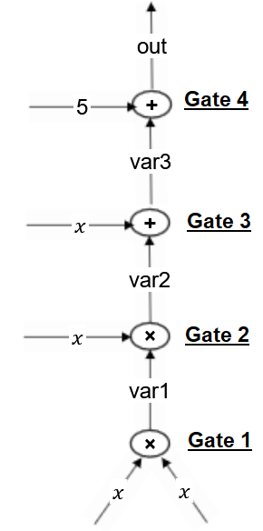
Next, we draw an arithmetic circuit of the above flattened program. As we see from the circut on the right, the circuit has 4 gates representing multiplication & addition operations & also has 5 variables & a constant “5”.

Let’s represent the variables in a solution vector S (also called as witness)

$S = [1, x, out, var1, var2, var3]$

$1$ is included as an element of the vector so as to represent constants.

We now convert the Arithmetic Circuit into a Rank-1 Constraint System (R1CS). A R1CS is a triplet of vectors (a, b, c), and a solution vector S, such that (a.S) * (b.S) = (c.S) where (.) is the dot-product. We will have 1 triplet/constraint for each of the arithmetic gates.

Gate 1

Now in the circuit diagram, let’s take the first gate which represents $var1 = x * x $

For the purpose of the conversion, we look at it as $x * x = var1$. The Left Hand Side represent the inputs & the Right Hand Side represents the output. We now represent it as 3 vectors, a, b & c. a & b are the LHS/input vectors & c is the RHS/output vector.

$a = [0, 1, 0, 0, 0, 0]$ (This represents the first term i.e. the $x$ before the multiplication operator. In the circuit, it represents the left side input going into the multiplication gate. Every element of the $a$ vector is 0 except the element corresponding to $x$ which has the value 1 - i.e. $1 * x$

$b = [0, 1, 0, 0, 0, 0]$ (This is the second term i.e. the $x$ after the multiplication operator - every element of the vector is 0 except the element corresponding to $x$)

$c = [0, 0, 0, 1, 0, 0]$ (This the output of the multiplication gate. Every element of the vector is 0 except the one corresponding to $var1$ which is the output of the gate)

Any solution vector which is correct will satify (a.S) * (b.S) = (c.S). Dot(.) represents the dot product of the 2 vectors.

Let’s try this out. We know the solution of the equation $x^3 + x + 5 == 35$ is $x = 3$. So substitute our solution vector $S = [1, x, out, var1, var2, var3]$ with the actual values based on $x = 3$

$var1 = x * x = 3 * 3 = 9$

$var2 = var1 * x = 9 * 3 = 27$

$var3 = var2 + x = 27 + 3 = 30$

$out = var3 + 5 = 30 + 5 = 35$

So $S = [1, 3, 35, 9, 27, 30]$

Dot product of two vectors $p = [p_1, p_2, …, p_n]$ and $q = [q_1, q_2, …, q_n]$ is defined as

$p . q = \sum_{i=1}^{n} = {p_1}{q_1} + {p_2}{q_2} + … + {p_n}{q_n}$

So $a.S = [0, 1, 0, 0, 0, 0].[1, 3, 35, 9, 27, 30]$

$a.S = 0 * 1 + 1 * 3 + 0 * 35 + 0 * 9 + 0 * 27 + 0 * 30 = 3$

Likewise $b.S = 3$ and $c.S = 9$

So $(a.S) * (b.S) = 3 * 3 = 9 = (c.S)$. So (a.S) * (b.S) = (c.S) is satisfied - this is a satisfied R1CS.

Gate 2

Let’s take the 2nd gate which represents $var1 * x = var2$

$a = [0, 0, 0, 1, 0, 0]$ (This represents the first term i.e. the $var1$ before the multiplication operator. Every element of the a vector is 0 except the element corresponding to $var1$)

$b = [0, 1, 0, 0, 0, 0]$ (This is the second term i.e. $x$ - every element of the vector is 0 except the element corresponding to $x$)

$c = [0, 0, 0, 0, 1, 0]$ (This the output of the multiplication operation- i.e. $var2$. Every element of the vector is 0 except the one corresponding to $var2$)

Gate 3

3rd gate is the addition gate which represents $var2 + x = var3$. The vectors for addition gates are derived differently. The equation is equivalent to $(var2 + x) * 1 = var3$. So the ‘a’ vector represents $var2 + x$, the ‘b’ vector represents ‘1’ & the ‘c’ vector represents var3

$a = [0, 1, 0, 0, 1, 0]$ (This represents $var2 + x$)

$b = [1, 0, 0, 0, 0, 0]$ (This represents $1$)

$c = [0, 0, 0, 0, 0, 1]$ (This represents $var3$)

Gate 4

Likewise, the 4th gate $var3 + 5 = out$ is equivalent to $(var3 + 5) * 1 = out$

$a = [5, 0, 0, 0, 0, 1]$ ($var3 + 5$)

$b = [1, 0, 0, 0, 0, 0]$ ($1$)

$c = [0, 0, 1, 0, 0, 0]$ ($out$)

Though we aren’t explicitly calculating & showing it here, (a.S) * (b.S) = (c.S) is satisfied for Gates 2, 3 & 4 also. We now have the complete R1CS with 4 constraints.

We can create a Matrix A by using each of ‘a’ vectors as a row in the Matrix. Likewise Matrices B & C.

The Complete Satisfied R1CS is

\(A = \begin{pmatrix} 0&1&0&0&0&0 \\ 0&0&0&1&0&0 \\ 0&1&0&0&1&0 \\ 5&0&0&0&0&1 \\ \end{pmatrix}\), \(B = \begin{pmatrix} 0&1&0&0&0&0 \\ 0&1&0&0&0&0 \\ 1&0&0&0&0&0 \\ 1&0&0&0&0&0 \\ \end{pmatrix}\), \(C = \begin{pmatrix} 0&0&0&1&0&0 \\ 0&0&0&0&1&0 \\ 0&0&0&0&0&1 \\ 0&0&1&0&0&0 \\ \end{pmatrix}\)

This along with our solution vector $S = [1, x, out, var1, var2, var3]$ forms our R1CS.

QAP

The next step is taking this R1CS and converting it into QAP form, which implements the exact same logic except using polynomials. We have 12 vectors of length 6. We have to transform these into 6 groups of 3 polynomials, each polynomial of degree 3.

A polynomial of degree n is defined by a minimum of n+1 points. Each column of A, B & C has 4 elements. So each such column can be converted into a polynomial of Degree 3. We use Lagrange’s Polynomial Interpolation to do this.

For e.g. 1st column of A is [0, 0, 0, 5] (transposed). We can consider each element as the y-coordinate corresponding to x = 1, 2, 3 & 4. So we get 4 sets of points - (1,0), (2,0), (3,0), (4,5) - this is an arbitrary interpretion we use to convert the R1CS into the QAP form.

We can find the polynomial passing through these 4 points using Lagrange Interpolation.

I am using sagemath to do this

R.<x> = PolynomialRing(RR)
points = [(1,0), (2,0), (3,0), (4,5)]
R.lagrange_polynomial(points)
$0.833333333333333 * x^3 - 5.00000000000000 * x^2 + 9.16666666666667 * x - 5.00000000000000$

So the first column of A has been transformed into a polynomial. We write the co-efficients of the polynomial as a vector/list

R.lagrange_polynomial(points).coefficients()
[-5.00000000000000, 9.16666666666667, -5.00000000000000, 0.833333333333333]

Likewise for the 2nd column of A

points = [(1,1), (2,0), (3,1), (4,0)]
R.lagrange_polynomial(points).coefficients()
[8.00000000000000, -11.3333333333333, 5.00000000000000, -0.666666666666667]

We have 3 matrices with 6 columns each, so we get 18 polynomials each with 4 coefficients.

A polynomials

$[-5.0, 9.166, -5.0, 0.833]$

$[8.0, -11.333, 5.0, -0.666]$

$[0.0, 0.0, 0.0, 0.0]$

$[-6.0, 9.5, -4.0, 0.5]$

$[4.0, -7.0, 3.5, -0.5]$

$[-1.0, 1.833, -1.0, 0.166]$

B polynomials

$[3.0, -5.166, 2.5, -0.333]$

$[-2.0, 5.166, -2.5, 0.333]$

$[0.0, 0.0, 0.0, 0.0]$

$[0.0, 0.0, 0.0, 0.0]$

$[0.0, 0.0, 0.0, 0.0]$

$[0.0, 0.0, 0.0, 0.0]$

C polynomials

$[0.0, 0.0, 0.0, 0.0]$

$[0.0, 0.0, 0.0, 0.0]$

$[-1.0, 1.833, -1.0, 0.166]$

$[4.0, -4.333, 1.5, -0.166]$

$[-6.0, 9.5, -4.0, 0.5]$

$[4.0, -7.0, 3.5, -0.5]$

This finishes the transformation of the problem to the QAP Form. Instead of checking the constraints in the R1CS individually, we can now check all of the constraints at the same time by doing a dot product check on the polynomials. This will be covered in a separate post.