The Sum-Check Protocol

$g$ is a $v$-variate polynomial defined over a Field $\mathbb F$.

The above equation sums $g$ over all possible Boolean inputs. The Prover ($\mathcal P$) claims that the sum is $u$. The Sum-Check protocol allows $\mathcal P$ to convince a Verifier ($\mathcal V$) that she has computed the sum correctly.

The steps in the protocol

$(1)$ $\mathcal P$ sends the value $u$ which she claims as the sum, to $\mathcal V$

$(2)$ $\mathcal P$ then sends a univariate polynomial $g_1$ in $x_1$ to $\mathcal V$. $\mathcal P$ claims it’s been created by summing $g$ in all variables except $x_1$ i.e. computing the following sum keeping $x_1$ free

$\qquad$ The right hand side above is the same expression as the right hand side in Expression (I) at the start except with the summation over $x_1$ removed.

$\qquad$ $Eq \space I$ results in a value in the left hand side because all variables were evaluated. Where $g_1$ becomes a univariate polynomial in $x_1$ instead of a value because $x_1$ is not summed for all values in $x_1 \in \lbrace 0,1 \rbrace$

$(3)$ $\mathcal V$ checks if $degree(g_1) <= degree(g)$. If not, $\mathcal V$ rejects the proof.

$(4)$ $\mathcal V$ then checks the one summation which was omitted by $\mathcal P$ while creating $g_1$. Doing that omitted summation should result in $u$

i.e. check if $\sum_{x_1 \in \lbrace 0,1 \rbrace} g_1(x_1) \stackrel {?}{=}u $

So he computes $g_1(0) + g_1(1)$ & checks if it sums to $u$.

If it does sum to $u$, then $\mathcal V$ can believe that $g$ also actually totals up to $u$ (which is the claim he is verifying) as long as he is sure that $g_1$ was indeed constructed the way described above (in Step $(2)$)

Let’s assume there is a polynomial $s_1$ which was actually created that way. i.e.

$\mathcal V$ has to verify that $g_1 = s_1$. He can do this by picking a random element $r_1 \in \mathbb F$ & verifying if $g_1(r_1) \stackrel {?}{=} s_1(r_1)$ (Schwartz-Zippel Lemma)

The complexity of creating $s_1$ & evaluating $s_1(r_1)$ isn’t much lesser than evaluating the original $g$ polynomial for all inputs & checking if it equals $u$. If $\mathcal V$ were to do this, he could as well herself calculate $g$ instead of getting it done by $\mathcal P$.

So instead, $\mathcal V$ checks if $s_1(r_1) \stackrel {?}{=} g_1(r_1)$ recursively as shown below.

$(5)$ $\mathcal V$ choses a random element $r_1 \in \mathbb F$ & sends it to $\mathcal P$

$(6)$ Just like $\mathcal P$ created $g_1$ by summing $g$ in all variables except $x_1$, now $\mathcal P$ creates $g_2$ by replacing $x_1$ in $g$ with the value $r_1$ & summing $g$ with $x_2$ free/unevaluated i.e. $x_1 = r_1$, $x_2$ free/unevaluated & but expanding all possible values of $x_3$ to $x_v$.

This creates a univariate polynomial $g_2(x_2)$. $\mathcal P$ sends $g_2$ to $\mathcal V$

$(7)$ $\mathcal V$ checks the degree of $g_2$ & rejects if not correct.

$(8)$ $g_2$ is built with $x_1 = r_1$ & $x_2$ kept free. So $\mathcal V$ needs to check if $g_1(x_1 = r_1) \stackrel {?}{=} g_2(x_2 = 0) + g_2(x_2=1)$

i.e. check if $g_1(r_1) \stackrel {?}{=} g_2(0) + g_2(1)$ & reject if not.

If it checks out, then all $\mathcal V$ needs to do is verify that $g_2$ indeed has been constructed correctly as described. So he continues the recursion as done below.

$(9)$ We have seen 2 rounds above already. Steps $(5)$ to $(8)$ are repeated for $j = 3$ to $j=v-1$

• $\mathcal V$ choses a random element $r_{j-1} \in \mathbb F$ & sends it to $\mathcal P$
• $\mathcal P$ creates the univariate polynomial $g_j(x_j)$ by keeping $x_j$ free and $x_1$ to $x_{j-1}$ fixed at $r_1$ to $r_{j-1}$ respectively

• $\mathcal V$ checks the degree & also if $g_{j-1}(r_{j-1}) \stackrel {?}{=} g_j(0) + g_j(1)$

$(10)$ In the last round, $\mathcal P$ sends $g_v(x_v)$ to $\mathcal V$. $\mathcal V$ checks degree & if $g_{v-1}(r_{v-1}) \stackrel {?}{=} g_v(0) + g_v(1)$

$(11)$ $\mathcal V$ then picks a random $r_v \in \mathbb F$ & evaluates $g(r_1, r_2, …, r_v)$. $\mathcal V$ also checks if $g_v(r_v) \stackrel {?}{=} g(r_1,r_2,…,r_v)$ & rejects if not.

If it checks out, then it means $g_{v-1}$ is the same polynomial as $s_{v-1}$ i.e. it has been constructed like the $\mathcal P$ said he constructed it. Which in turn means $g_{v-2}$ is the same as $s_{v-2}$. As we keep unrolling, finally, it proves that $g_1$ is equal to $s_1$ which proves the original summation sums up to $u$. This ends the proof.

The $\sharp$SAT Problem

We will run through the Sum-Check protocol using a $\sharp SAT$ example

$(x_1 \space \& \space x_2) \space \& \space(x_3 \space | \space x_4)$

In $\sharp SAT$ you have to check for all possible different combinations of $x_1, x_2, x_3, x_4$ & count how many combinations end up satisfying the above boolean circuit/formula i.e. evaluate to TRUE(1).

Any boolean formula can be arithmetized & converted into a function by replacing

• $A\space \& \space B$ with $A * B$
• $A\space | \space B$ with $(A + B) - (A*B)$
• $! A$ with $1 - A$

Arithmetizing the above boolean circuit gives us $g(x_1, x_2, x_3, x_4) = (1-x_1) x_2 ((x_3 + x_4) - x_3x_4)$

We will walk through the protocol using a sagemath program.

We will operate in a Finite Field $\mathbb F_{97}$. First $\mathcal P$ evaluates $g$ for all possible values of $x_1,x_2,x_3,x_4$ i.e.

F97 = GF(97)
R97.<x1,x2,x3,x4> = PolynomialRing(F97)
g = R97((1-x1)*x2*((x3+x4)-x3*x4))
sum = 0

for a1 in [0,1]:
    for a2 in [0,1]:
        for a3 in [0,1]:
            for a4 in [0,1]:
                sum = sum + g(a1,a2,a3,a4)

Sum evaluates to $3$

$\mathcal P$ creates a univariate polynomial in $x_1$

g1 = R97(0)
for a2 in [0,1]:
    for a3 in [0,1]:
        for a4 in [0,1]:
           g1 = g1 + g(x1,a2,a3,a4)

If you print out $g_1$,

$g_1(x_1) = -3x1 + 3$

$\mathcal V$ computes $g_1(x_1=0) + g_1(x_1=1)$ & checks if it evaluates to 3.

$\mathcal V$ picks random number $r_1 \in \mathbb F_{97}$, $r_1=25$ & sends it to $\mathcal P$

$\mathcal P$ keeps $x_1=r_1$ & creates the next univariate polynomial $g_2$ keeping $x_2$ free.

r1 = 25
g2 = R97(0)
for a3 in [0,1]:
    for a4 in [0,1]:
       g2 = g2 + g(r1,x2,a3,a4)

This creates $g_2(x_2) = 25x_2$ & is sent to $\mathcal V$

$\mathcal V$ checks if $g_1(x_1=r_1) \stackrel {?}{=} g_2(x_2=0) + g_2(x_2=1)$, which checks out - both LHS & RHS are 25.

Then,

r2 = 6
g3 = R97(0)
for a4 in [0,1]:
   g3 = g3 + g(r1,r2,x3,a4)

$g_3(x_3) = -47x3 - 47$

$g_2(x_2=r_2) = g_3(x_3=0) + g_3(x_3=1) = -44$ - checks out.

r3 = 11
g4 = R97(g(r1,r2,r3,x4))

$g_4(x_4) = -15x4 - 32$

$\mathcal V$ picks $r_4=3$

$g_4(x_4=r_4) = -3$

$g(r1,r2,r3,r4) = 94$ (same as $-3 \bmod 97$)

So again checks out & the proof is done.

Extension Polynomials and Multilinear Extensions

Let’s say we have a vector $a = [11,7,23,14]$ & we want to encode it into a univariate polynomial, one of the ways to do is to first consider these elements as y-coordinates of points corresponding to $x \in [0,1,2, 3]$ like we did in QAP.

We start with a map $f: \lbrace 0,1,2,3 \rbrace \mapsto \lbrace 11,7,23,14 \rbrace$ & we then use Lagrange Interpolation of the points $[(0,11),(1, 7),(2, 23), (3, 14)]$ to create the polynomial $\tilde f(x) = 41x^3 + 81x^2 + 68x + 11$.

Though we were interested only in inputs of $0,1,2,3$, the polynomial can take all inputs in $\mathbb F_{97}$ i.e. $\tilde f(0) = 11, \tilde f(1) = 7, \tilde f(2) =23, \tilde f(3) = 14, \tilde f(4)= 32, \tilde f(5) = 32, …, \tilde f(95) = 65, \tilde f(96)=80$

We started with a vector $a = [11,7,23,14]$ and encoded it into a polynomial whose domain can be considered as a much larger vector $a’ = [\mathit{11, 7 , 23,14}, 32,32,…,65,80]$

This polynomial $\tilde f$ maps $\mathbb F_{97} \mapsto \mathbb F_{97}$

Hence the polynomial $\tilde f$ is called an extension of the original map/function which mapped just those 4 elements.

If $|a|$ is much smaller than $|a’|$ (i.e size of field is much larger), then it’s called a low degree extension (numercial examples in this post do not operate in a very large field, we operate in $\mathbb F_{97}$ for ease of understanding - so these examples don’t actually generate a low degree extension)

The above was a Univariate Polynomial. A Multivariate Polynomial which has a maximum degree of $1$ in each of it’s variables is called as Multilinear Polynomial. For e.g. $2xy + 3x + y$ is a multilinear polynomial but $2x^2 + 3xy + 5$ isn’t multilinear.

For the univariate case, we considered functions/maps whose domain was $\lbrace 0,1,2, …, n-1\rbrace$ which mapped to $\mathbb F$ & we interpolated their extension. In the multivariate case, we will look at functions/maps whose domain is $\lbrace 0, 1 \rbrace^v$ & map it to $\mathbb F$.

In the univariate case, if we had a vector of $n$ values which we wanted to encode in our univariate polynomial, we picked the input domain as $\lbrace 0,1,…,n-1\rbrace$ - like for $a = [11,7,23,14]$ of size $4$, we used the input domain $\lbrace 0, 1, 2,3 \rbrace$. In the multivariate case, for encoding a vector of size $n$, we pick $v=log\space n$ & use $\lbrace 0, 1 \rbrace^v$ as the input domain. $\lbrace 0,1 \rbrace^v$ is called as the $v$-dimensional Boolean Hypercube.

Lagrange Interpolation of a Multilinear Extension (MLE) Polynomial

Let’s encode the same vector $\lbrace 11,7,23,14 \rbrace$ into a multilinear polynomial.

Like before, we start with a map $f: \lbrace 0,1,2,3 \rbrace \mapsto \lbrace 11,7,23,14 \rbrace$.

Our input domain size is 4, so our $v=log(4)=2$. So we use $\lbrace 0, 1 \rbrace^2$. This has 4 values - $0, 1, 2, 3$ - expressing this in binary it becomes $00, 01, 10, 11$. So each element of the input domain has 2 bits - i.e. so we need a bivariate polynomial $\tilde f(x_1,x_2)$ where $x_1$ will take the value of the first bit & $x_2$ the 2nd bit. In general, $x_1$ will take the value of the Most Significant Bit (MSB) & the last $x_v$ will be the LSB. So if we start with a vector of size $n$, we will end up with a $v$-variate polynomial where $v=log\space n$

For the interpolation, we first calculate the Multilinear Lagrange Basis Polynomials using this formula

$w_i$ is the current bit - for e.g. for the input bitstring $10$, $w_1 = 1, w_2 = 0$

Let’s create $L_{00}$ corresponding to input $0$ (bitstring $00$)

$L_{00} = \prod_{i=1}^2 (x_iw_i + (1-x_i)(1-w_i))$

$\qquad = (x_1w_1 + (1-x_1)(1-w_1)) \cdot (x_2w_2 + (1-x_2)(1-w_2))$

Here, $w_1 = 0$ & $w_2 = 0$

$L_{00} =(1-x_1).(1-x_2) = 1-x_2-x_1+x_1x_2$

For $L_{01}$, $w_1 = 0$ & $w_2 = 1$

$L_{01} = (1-x_1).(x2) = x_2 -x_1x_2$

$L_{10} = x_1 - x_1x_2$

$L_{11} = x_1x_2$

Using the Lagrange basis Polynomials, we can now calculate the Multilinear extension for our map $f: \lbrace 1,2,3, 4 \rbrace \mapsto \lbrace 11,7,23,14 \rbrace$ using the below formula

$\tilde f(x_1,x_2) = f(0)\cdot L_{00} + f(1)\cdot L_{01} + f(2) \cdot L_{10} + f(3) \cdot L_{11}$

$\qquad = 11\cdot (1-x_2-x_1+x_1x_2 ) + 7\cdot (x_2 -x_1x_2) + 23\cdot (x_1 - x_1x_2)+ 14 \cdot (x_1x_2)$

$\qquad = 11-11x_2-11x_1+11x_1x_2 + 7x_2 -7x_1x_2 + 23x_1 - 23x_1x_2 + 14x_1x_2$

$\boldsymbol{\tilde f(x_1,x_2) = 11 + 12x_1 - 4x_2 -5x_1x_2}$

The map $f$ mapped only the input domain $[0,1,2,3]$ which is same as $(x_1,x_2) = [(0,0), (0,1), (1,0), (1,1)]$, but $\tilde f$ can actually be evaluated for all possible $x_1 \& x_2\space’s \in F_{97}$ - hence if is a multilinear extension of the map.

Here is a sage program do the same thing we did manually above

v = 2 #v-dimensional Boolean hypercube

fmap = [11, 7, 23, 14]

F97 = GF(97)
Lw = [] # Lagrange Basis 
R97 = PolynomialRing(F97, v, [f"x{i}" for i in range(1, v+1)])

for i in range(2^v):
    b=Integer(i).digits(2, None, v) # pad(ZZ(i).binary(),v)
    g = R97(1)

    for j in range(v):
        xi = R97.gen(j)
        wi = b[v-1-j]
        g = g* (xi * wi + (1-xi)*(1-wi))

    Lw.append(g)

#MLE
f = R97(0)
for i in range(2^v):
    f = f+ fmap[i]*Lw[i]

print("MLE = " + str(f))

Note: Our $g$ polynomial, on which we run the Sum-Check Protocol need not be a multilinear polynomial. In some examples, you will see that it will be a product of multilinear polynomials & the product may not be multilinear. But in most practical cases, $g$ will have a degree at most of $2$ or $3$ in each of it’s variables.

Optimisations

The input to $\mathcal V$ sent by $\mathcal P$ is the values of the map $f[w]\space\forall\space w\space\in\space2^v$. In the Sum-Check Protocol, the verifier has to only evaluate the MLE once at the end at a random point. So it may not be actually necessary for $\mathcal V$ to first compute the MLE & then evaluate it. $\mathcal V$ can instead directly evaluate the MLE without ever forming the polynomial.

Let us say that $\mathcal V$ has to evaluate the MLE at random value $r = r_1, r_2, …, r_v$, he can first compute Lagrange Basis Polynomials using $Eq II$ in the above section on MLE’s using $x_1 = r_1, x_2 = r_2, …$ & then use $Eq III$ directly with the $f$s and the Lagrange Basis polynomials to evaluate the MLEs.

Let’s take an example.

$\mathcal P$ sends $\mathcal V$ the map $f : \lbrace 0,1 \rbrace ^3 \mapsto \mathbb F$ given by $f(0,0,0) = 1, f(0,1,0) = 2, f(1,0,0) = 3, f(1,1,0) = 4, f(0,0,1) = 5, f(0,1,1) = 6, f(1,0,1) = 7, f(1,1,1) = 8$

$\mathcal V$ has to evaluate the MLE $\tilde f$ at a random point $r = [2,4,6]$ i.e. evaluate $\tilde f(2,4,6)$

v = 3
fmap = [1,2,3,4,5,6,7,8]
r = [2, 4, 6] # Random Point
F97 = GF(97)
sum = 0

for i in range(2^v):
    b=Integer(i).digits(2, None, v) 
    # i'th Lagrange Base 
    Lw = R97(1)

    for j in range(v):
        wi = b[v-1-j]
        
        # Eq II to form the Lagrange Basis
        Lw = Lw* (r[j] * wi + (1-r[j])*(1-wi))
    
    #Eq III 
    sum = sum + fmap[i] * g
print(sum)

The above program will print $23$. So $\mathcal V$ has successfully evaluated the MLE without actually forming the MLE.

If you look at the above program carefully, you will notice that it calculates does the multiplications $(1-r_1) \cdot (1-r_2)$, $(r_1\cdot r_2)$, $(1-r_1)\cdot(r_2)$ multiple times. As $v$ becomes larger the number of multiplications which get repeated creates a huge inefficiency. We can use dynamic programming/memoization to optimise it (If you are not familiar with this concept, you can take a look at this video - Dynamic Programming Tutorial with Fibonacci Sequence )

Let’s first assume $v = 1$ & calculate $L_0$ & $L_1$

$L_0 = (1-r1) = -1$

$L_1 = (r1) = 2$

Next with $v = 2$

$L_{00} = L_0 \cdot (1-r_2) = 3$

$L_{01} = L_0 \cdot r_2 = -4$

$L_{10} = L_1 \cdot (1-r2) = -6$

$L_{11} =L_1 \cdot r_2 = 8$

With $v=3$

$L_{000} = L_{00} \cdot (1-r_3) = -15$

$L_{001} = L_{00} \cdot r_3 = 18$

$L_{010} = L_{01} \cdot (1-r_3) = 20$

$L_{011} = L_{01} \cdot r_3 = -4 \cdot 6 = -24$

$L_{100} = L_{10} \cdot (1-r_3) = -4 \cdot (-6) = 30$

$L_{101} = L_{10} \cdot r_3 = -6 \cdot 6 = -36$

$L_{110} = L_{11} \cdot (1-r_3) = 8 \cdot -5 = -40$

$L_{111} = L_{11}\cdot(r_3) = 8 \cdot 6 = 48$

Now we can evaluate the $\tilde f(2,4,6)$ as

$ L_{000}\cdot f(0) + L_{001}\cdot f(1) + L_{010}\cdot f(2) + L_{011}\cdot f(3) + L_{100}\cdot f(4) + L_{101}\cdot f(5) + L_{110}\cdot f(6) + L_{111}\cdot f(7)$

which evaluates to 23

The same thing in a program

v = 3
fmap = [1,2,3,4,5,6,7,8]
r = [2, 4, 6]
F97 = GF(97)
Lw = [[1-r[0],r[0]]]

for j in range(1,v):
    Lwt = [F97(1)]*2^(j+1)

    for i in range(2^(j+1)): 
        b = f'{i:b}'.zfill(j+1)
        lsb = b[j:j+1]
        rest =  b[0:j]
        
        if (lsb == "0"):
            Lwt[i] = R97(Lw[j-1][Integer('0b' + rest)]* (1-r[j]))
        else:
            Lwt[i] = R97(Lw[j-1][Integer('0b' + rest)]* r[j])
        
    Lw.append(Lwt)

# Compute f(2,4,6)
sum = 0
for i in range(2^v):
    sum = sum + fmap[i]*Lw[v-1][i]

print(sum)

Encoding the Adjacency Matrix of a Graph

let’s consider a Graph $G = (U,E)$ where $E$ the set of $k$ edges & $U$ is the set of $n$ vertices numbered from $0$ to $n-1$ i.e. $U = \lbrace 0, 1, 2, …, n-1\rbrace$.

The Adjacency Matrix for this graph is a square matrix $A$ of size $n\times n$ where we interpret the row & column numbers of elements as vertex numbers. If there is an edge between vertex $i$ & vertex $j$ the Matrix Element $A_{ij} = 1$, else $0$.

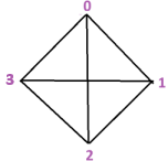
Lets take this graph.The adjacency matrix will be

The adjacency matrix is a map $f: (row, col) \mapsto \lbrace 0, 1 \rbrace$

Since maximum row or column number is $4$, it can each be represented by $log(n)$ bits i.e.

$f: \lbrace 0, 1 \rbrace^{2} \times \lbrace 0, 1 \rbrace^{2} \mapsto \lbrace 0, 1 \rbrace$

We will interpolate this to an MLE $\tilde f(row,col)$. As said earlier, each row number & column number will take two bits to represent.

i.e. $\tilde f ((r_0,r_1),(c_0, c_1 ))$, where $r_0$ & $r_1$ are the bits of the row number. This is $\tilde f (r_0,r_1,c_0,c_1)$ - i.e. the MLE takes 4 parameters which can be represented by the 4 variables $x_1, x_2, x_3, x_4$.

We will use our earlier program to interpolate the MLE with the following values of $fmap$ & $v$

$fmap = [0,1,1,1,1,0,1,1,1,1,0,1,1,1,1,0]$

$v = 4$ (2 bits each for row & column number)

Running the program, we get

$\tilde f = -4x_1x_2x_3x_4 + 2x_1x_2x_3 + 2x_1x_2x_4 + 2x_1x_3x_4 + 2x_2x_3x_4 - x_1x_2 - 2x_1x_3 - x_2x_3 - x_1x_4 - 2x_2x_4 - x_3x_4 + x_1 + x_2 + x_3 + x_4$

Caveats in the above example

A graph with $4$ nodes will have an Adjacency Matrix of size $4\times4$ & the row & column numbers will go from $0$ to $3$, so they can be represented in $2$ bits each, so any element in the matrix can be represented as (row, column) with 4 bits which works fine. But it’s not always so seamless.

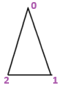
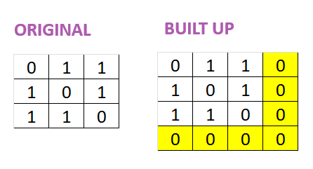
Let’s take for example the Adjacency Matrix for this 3 vertex graph. It’s a $3\times 3$ matrix, so row, col numbers are from $0$ to $2$, this still needs $2$ bits. So totally $4$ bits will be needed to represent each element. So we need to convert the $3\times 3$ Adjacency matrix into a $4\times4$ matrix by setting the extra elements as $0$ before we interpolate it into an MLE.

Below you can see how the matrix can be built up into a $4\times 4$ matrix. The elements in yellow are extra elements we added.

In general, if you need $v$ bits to represent each element & interpolate a $v$-variate polynomial, then you will need to build up the matrix to have $2^{v}$ elements i.e. a $n\times n$ matrix where $n = \sqrt(2^v)$

Counting Triangles

Now, we will use our MLE to count the number of triangles in our 4 vertex graph (Note this is our first graph - the 4-vertex one & not the 3-vertex graph we discussed after that). We have already computed the MLE for this.

$\tilde f = -4x_1x_2x_3x_4 + 2x_1x_2x_3 + 2x_1x_2x_4 + 2x_1x_3x_4 + 2x_2x_3x_4 - x_1x_2 - 2x_1x_3 - x_2x_3 - x_1x_4 - 2x_2x_4 - x_3x_4 + x_1 + x_2 + x_3 + x_4$

Consider any 3 vertices out of the 4 - let’s call them $a,b,c$. These 3 vertices will form a triangle if & only if there is an edge between $a$ & $b$, and an edge between $b$ & $c$ & another between $c$ & $a$. Which means, only if all three of $\tilde f(a,b),\tilde f(b,c), \tilde f(c,a)$ evaluate to 1 - i.e. only if

$\tilde f(a,b)\cdot \tilde f(b,c)\cdot \tilde f(c,a) = 1$

Even if one of the two vertices out of the three doesn’t have an edge between them, then that evaluation of $\tilde f$ with those edges as params will be $0$ i.e. the above multiplication will result in $0$. So the above equation can be used to count the number of triangles in a graph. However, the triangle formed by $3$ edges $(ab)(bc)(ca)$ is the same as that formed by $(ba)(cb)(ac)$ - each triangle can be represented in 6 different ways by $\tilde f$. So to get the count of the total number of triangles in the graph, we have to divide by $6$.

$\frac {1}{6} \times \sum_{a \in \lbrace 0, 1 \rbrace^{2}} \sum_{b \in \lbrace 0, 1 \rbrace^{2}} \sum_{c \in \lbrace 0, 1 \rbrace^{2}} \tilde f(a,b)\cdot \tilde f(b,c) \cdot \tilde f(c,a)$

When $\mathcal P$ computes the above, she will get the answer $24$. And $\frac {1}{6}\times 24 = 4$

So count of triangles in our graph is $4$ which can also be verified visually for a small graph like our 4-vertex graph.

$\mathcal P$ proves this to $\mathcal V$ using the Sum-Check protocol. Since we have already gone through all the steps of the protocol with other examples, I am not discussing each step here but only ones where we do things differently.

• $\mathcal P$ doesn’t need to multiply the 3 $\tilde f$’s to create a $g$ before evaluating it or running the Sum-Check protocol. Actually multiplying the $\tilde f$’s makes it more complicated. She can instead evaluate the 3 $\tilde f$’s & then multiply the evaluations to get $24$ which is then divided by $6$ to get $4$. For e.g.

sum = 0
for a1 in range(2):
  for a2 in range(2):
    for a3 in range(2):
      for a4 in range(2):
        for a5 in range(2):
          for a6 in range(2):
             sum = sum + f(a1, a2, a3, a4) * f(a3, a4, a5, a6) * f(a5, a6, a1, a2)
      
print(sum)

• In step $2$, $\mathcal P$ has to send the univariate polynomial $g_1$ to $\mathcal V$. Again, this can be done without the verifier first creating a $g$.

g1 = R97(0)
for a2 in range(2):
  for a3 in range(2):
    for a4 in range(2):
      for a5 in range(2):
        for a6 in range(2):
          g1 = g1 + f(x1,a2,a3,a4) * f(a3,a4,a5,a6) * f(a5,a6,x1,a2)

This gives us $g_1 = -4x1^2 + 4x1 + 12$

But there is an even better way to do this. $g_1$ is a polynomial of at most degree $2$, so instead of creating $g_1$ & sending it, $\mathcal P$ can instead send evaluations of $g_1$ at 3 points - i.e. values of $g_1(0)$, $g_1(1)$, $g_1(2)$ & $\mathcal V$ can recreate $g_1$ himself at his end using Lagrange Interpolation for univariate polynomials.

a1 = [0,1,2]
sum = [0,0,0]

for i in range(len(a1)):
  for a2 in range(2):
    for a3 in range(2):
      for a4 in range(2):
        for a5 in range(2):
          for a6 in range(2):
            sum[i] = sum[i] + f(a1[i],a2,a3,a4) * f(a3,a4,a5,a6) * f(a5,a6,a1[i],a2)
            
print(sum)

This prints out $[12, 12, 4]$ - i.e. $g_1(0) = 12, g_1(1) = 12, g_1(2) = 4$

When $\mathcal V$ uses univariate Lagrange Interoplation, then he will get the same $g_1 = -4x1^2 + 4x1 + 12$

In all the steps where $\mathcal P$ has to send a univariate $g_i$, she instead sends the appropriate number of evaluations instead.

Note that the above program has many calculations which are redone repeatedly & hence can be optimized further by dynamic programming.

In the final step of the protocol, $\mathcal V$ has to compute $\tilde f(r_1,r_2)\cdot \tilde f(r_2, r_3)\cdot \tilde f(r_3, r_1)$ where each $r_i$s is a vector of random values - as seen earlier each of the 3 are vectors of size $\log n = v$. We pick $r_1, r_2, r_3 \in \mathbb F^{\log n} \times \mathbb F^{\log n} \times \mathbb F^{\log n}$. In our case, $\log n = v = 2$, so $\mathcal V$ has to pick 6 random numbers say $r_{11}, r_{12}, r_{21}, r_{22}, r_{31}, r_{32}$ - i.e. $r_1$ is the vector $\lbrace r_{11}, r_{12}\rbrace$, $r_2$ the second two and so on. $\mathcal V$ then computes $\tilde f (r_{11}, r_{12}, r_{21}, r_{22}) \cdot \tilde f (r_{21}, r_{22}, r_{31}, r_{32}) \cdot \tilde f (r_{31}, r_{32}, r_{11}, r_{12}) $ which can be done in time linear to the size of the input Matrix.

This post is based on Justin Thaler’s Book Proofs, Arguments, and Zero-Knowledge