Notes

$\mathbb F_p$ is a Finite Field. We use an Elliptic Curve $E(\mathbb F_p)$ over this field. The order of the curve is $q$ & the discrete log problem is hard in the Group of the Curve. When we sample any random numbers in this post, please assume it’s sampled from $\mathbb F_q$.

The Prover is $\mathcal P$ & the Verifier $\mathcal V$.

Prerequisites

Pedersen Commitments

The basic Pedersen Commitment has been covered in the earlier Monero post - Privacy and Anonymity in Monero .

Pedersen Vector Commitments

I use the following notations for vectors. The arrow on top denotes that it is a vector & not just a single value

$\overrightarrow m = [m_0, m_1, m_2, m_3]$

For convenience, I represent vectors horizontally in this post except in case of vector polynomials where I represent the vector coefficients vertically.

I represent a vector of exponentiated scalars as

$\overrightarrow {a^n} = [a^0, a^1, a^2, …, a^n]$

Pedersen Commitments can be extended to commit a vector of elements.

The Pedersen Commitment for the vector $\overrightarrow m$ is

$C_m = m_0 G_0 + m_1 G_1 + m_2 G_2+ m_3 G_3 + bB$

Here $b$ is the blinding factor & $B, G_0, G_1, G_2, G_3$ are all generators & the relation between the different Generators is not known.

The above commitment can also be written as

$C_m = \overrightarrow m \overrightarrow G + bB$

where $\overrightarrow G = [G_0, G_1, G_2, G_3]$ & is called the “basis” committing $\overrightarrow m$

This can also be extended for committing multiple vectors in a single commitment

$C_{mn} = \overrightarrow m \overrightarrow H + \overrightarrow n \overrightarrow G + bB$

Pedersen Polynomial Commitments

Throughout this post, I present protocols & proofs as interactive ones, but they would be used with the Fiat-Shamir heuristic to make them non-interactive.

$p(x) = c_0 + c_1 x + c_2 x^2$

In order to commit to the polynomial, $\mathcal P$ makes a separate commitment to each of the coefficients & sends them to $\mathcal V$.

$C_0 = c_0G + b_0 B$

$C_1 = c_1G + b_1 B$

$C_2 = c_2G + b_2 B$

where $b_0, b_1, b_2$ are randomly sampled blinding factors

$\mathcal P$ can do a zero knowledge opening of this polynomial commitment with the following Evaluation Proof

• $\mathcal V$ randomly samples $u$ & sends it to $\mathcal P$.

• $\mathcal P$ evaluates $p(x)$ at $u$, $p_u = p(u) = p_0 + p_1u + p_2u^2$.

• $\mathcal P$ also computes $b = b_0 + b_1 u + b_2 u^2$.

• $\mathcal P$ sends $p_u$ & $b$ to $\mathcal V$.
• $\mathcal V$ checks if $C_0 + C_1u + C_2u^2 \stackrel {?}{=} p_uG + bB$.

If it is, then $\mathcal V$ accepts that the evaluation $p(u)$ is $p_u$ & that $\mathcal P$ knows the polynomial $p(x)$ by the Schwartz-Zippel Lemma.

This works because

$p_uG + bB\space= (p_0 + p_1u + p_2u^2)G + (b_0 + b_1 u + b_2 u^2)B$

$\qquad\qquad = p_0G + (p_1G + b_1B)u + (p_2G + b_2B )u^2 + b_0B)$

$\qquad\qquad = C_0+ C_1u+C_2u^2$

Zero Knowledge Polynomial Product Proof

$l(x) = l_0 + l_1x$

$r(x) = r_0 + r_1x$

$t(x) = l(x) r(x) = (l_0 + l_1x)(r_0 + r_1x)$

$\qquad = l_0 r_0 + (l_0 r_1 + l_1 r_0)x + l_1 r_1 x^2$

Let $t_0 = l_0 r_0, t_1 = (l_0 r_1 + l_1 r_0), t_2 = l_1 r_1 $

$t(x) = t_0 + t_1x + t_2x^2$

$\mathcal P$ wants to prove that $t(x) = l(x)r(x)$

To prove this, she provides these proofs.

$1)$ Evaluation Proofs for $t(x), l(x)$ & $r(x)$ separately using the method used in the previous section.

• $\mathcal P$ sends commitments to the coefficients of each of the 3 polynomials (total 7 commitments).

• $\mathcal V$ sends random $u$.

• $\mathcal P$ evaluates $l_u = l(u), r_u = r(u), t_u = t(u)$. $\mathcal P$ sends these values to $\mathcal V$.

• $\mathcal V$ checks the evaluation proof for each of the 3 polynomials using the method described in the earlier section & rejects the proof it doesn’t verify.

$2)$ Proof that evaluation of $t$ at a random point is equal to the product of the evaluations of $l$ & $r$ at the same point.

• $\mathcal V$ checks if $t_u \stackrel {?}{=} l_u r_u$ and accepts the proof if it is.

This involves $\mathcal P$ sending 7 commitments & $\mathcal V$ checking 4 equalities. This can be optimized as below.

Optimized Proof

In the earlier section, $\mathcal V$ verified $l(x)$ & $r(x)$ separately, but this can be optimized by verifying both in a single step.

Commitment to $l(x)$ can be looked at as a commitment to the constant term (the term $x^0$ - i.e. the co-efficient with no $x$ terms) linearly combined with the linear term (term with $x^1$) combined in a linearly independent way.

$C_{l(x)} = C_{l_0} + C_{l_1}x$

$C_{r(x)} = C_{r_0} + C_{r_1}x$

Both can be combined as

$S = C_{l(x=u)} + C_{r(x=u)} = C_{l_0} +C_{r_0} + C_{l_1}u + C_{r_1}u = C_0 + C_1u$

So instead of 4 commitments, $\mathcal P$ makes 2 commitments for $l$ & $r$.

$C_0 = l_0 G + r_0 H + b_0 B$

$C_1 = l_1 G + r_1 H + b_1 B$

Commitments for $t(x)$ remain like before.

$C_{t_0} = l_0 r_0 G + b_{t_0}B$

$C_{t_1} = (l_0 r_1 + l_1 r_0) G + b_{t_1}B$

$C_{t_2} = l_1 r_1 G + b_{t_2}B$

$\mathcal P$ sends 5 commitments to $\mathcal V$.

$\mathcal V$s sends $u$ like before & $\mathcal P$ evaluates $l, r, t$ at & $u$ and sends the evaluations $l_u, r_u$ & $t_u$ to $\mathcal V$. She also sends $b_t = b_{t_0} + b_{t_1}u + b_{t_2}u^2$ & $b_{lr} = b_0 + u$.

$\mathcal V$ computes

$S = C_0 + C_1\space u$

$\mathcal V$ checks if $S \stackrel {?}{=} l_u G +r_eH + b_{lr}B$ - which is equivalent to checking both $l(x)$ & $(x)$.

This works if $\mathcal P$ is honest because

$C_0 + C_1\space u = l_0G + r_0H + b_0B+ l_1uG + r_1uH + b_1uB$

$\qquad\qquad = (l_0 + l_1u)G + (r_0 + r_1u)H + (b_0 + b_1u)B$

$\qquad\qquad = l_u G +r_uH + b_{lr}B$

Other checks remain the same as before i.e. evaluation proof of $t(x)$ & proof that $t_u = l_u r_u$.

Inner Product

Two vectors,

$\overrightarrow m =[ m_0, m_1, m_2]$

$\overrightarrow n =[ n_0, n_1, n_2]$

The Inner Product of these 2 vectors is

$<\overrightarrow m, \overrightarrow n> = m_0 n_0 + m_1 n_1 + m_2 n_2 $

i.e. the corresponding elements of the 2 vectors are multiplied with each other & then added up. Note that the output of an inner product is a scalar/single value & not a vector. An inner product is also called a dot product in some contexts.

A Vector Commitment can also be represented as an Inner Product.

$C_m = bB + m_0\space G_0 + m_1\space G_1 + m_2\space G_2+ m_3\space G_3$

The above can be written as an inner product.

$C_m= bB + <\overrightarrow m, \overrightarrow G>$

A Polynomial $p(x) = p_0 + p_1x + p_2x^2 + … + p_nx^n$

can be written as $p(x) = <\overrightarrow p, \overrightarrow {x^n}>$ where $\overrightarrow p$ is the vector of coefficients $[p_0, p_1, p_2, …, p_n]$.

The evaluation of $p$ at $u$ would be $<\overrightarrow p, \overrightarrow{u^n}>$.

Hadamard Product

A Hadamard product of 2 vectors is represented as

$\overrightarrow m \circ \overrightarrow n = [m_0 n_0, \space\space m_1 n_1, \space\space m_2 n_2]$

Note that unlike the inner product, the output of the Hadamard product is a vector. When the elements of the Hadamard product output are added together, you get the Inner Product.

Since the output a Hadamard Product is a vector, a Hadamard product can be an input to an inner product, i.e.

$< \overrightarrow m \circ \overrightarrow n, \space \space \overrightarrow a>$

If the hadamard product of $ \overrightarrow m$ & $\overrightarrow n$ gives us the vector $\overrightarrow p = [m_0 n_0, \space\space m_1 n_1, \space\space m_2 n_2 ]$, then the Inner Product $<\overrightarrow m \circ \overrightarrow n , a>$ would be the same as $<\overrightarrow p, \overrightarrow a>$.

Product Algebra

Some rearranging of Inner Products & Hadamard Products which we will be using later.

• $\quad <\overrightarrow m,\space\space \overrightarrow p+\overrightarrow q> = m_0 (p_0+q_0) + m_1 (p_1+q_1) + m_2 (p_2+q_2) $

$\qquad = m_0 p_0+m_0 q_0 + m_1 p_1+m_1 q_1 + m_2 p_2+m_2 q_2 $

$\qquad = (m_0 p_0 + m_1 p_1 + m_2 p_2 ) + (m_0 q_0 + m_1 q_1 + +m_2 q_2)$

$\qquad = <\overrightarrow m, \overrightarrow p> + <\overrightarrow m, \overrightarrow q>$

• The above also means

$\quad <\overrightarrow m+\overrightarrow n, \overrightarrow p + \overrightarrow q> = <\overrightarrow m+\overrightarrow n,\overrightarrow p> + <\overrightarrow m+\overrightarrow n,\overrightarrow q> = <\overrightarrow m, \overrightarrow p> + <\overrightarrow n,\overrightarrow p> + <\overrightarrow m, \overrightarrow q> + <\overrightarrow n,\overrightarrow q>$

• We can also rearrange an Inner product as an Inner Product containing a Hadamard Product.

$\quad <\overrightarrow m,\overrightarrow n> = m_0 n_0 + m_1 n_1 + m_2 n_2$

$\qquad = 1^0 ( m_0 n_0) + 1^1 ( m_1 n_1) + 1^2 ( m_2 n_2) $

$\qquad = <\overrightarrow {1^n}, \overrightarrow m\circ \overrightarrow n>$

• Consider a scalar $s$,

$\qquad s <\overrightarrow m, \overrightarrow n> = s (m_0 n_0 + m_1 n_1 + m_2 n_2 )$

$\qquad = (s m_0)n_0 + (s m_1) n_1 + (s m_2) n_2$

$\qquad = <s\overrightarrow m, \overrightarrow n> = <\overrightarrow m, s\overrightarrow n>$

• $\overrightarrow m = [m_0, m_1, m_2, m_3] = [m_0.1^0, m_1.1^1, m_2.1^2, m_3.1^3] = \overrightarrow m \circ \overrightarrow 1^4$

$\qquad$ So, $\overrightarrow m=\overrightarrow m \circ \overrightarrow 1^4$

• $\overrightarrow m \circ s1^4 = s\overrightarrow m\circ 1^4 = s\overrightarrow m$

• Consider $\overrightarrow m$ is made of two halves $\overrightarrow m_L$ & $\overrightarrow m_R$

$\qquad$ i.e. $\overrightarrow m = [m_0,m_1, m_2, m_3]$

$\qquad \overrightarrow m_L = [m_0, m_1]$ & $\overrightarrow m_R = [m_2, m_3]$

$\qquad$ and likewise $n_L$ & $n_R$ are the two halves of $n$,

$\qquad$ If concatenation is represented by $\oplus$, then (Note that $\oplus$ is different than $+$)

$\qquad \overrightarrow m = \overrightarrow m_L \oplus \overrightarrow m_R$ & $\overrightarrow n = \overrightarrow n_L \oplus \overrightarrow n_R$

then $<\overrightarrow m, \overrightarrow n> = m_0 n_0 + m_1 n_1 + m_2 n_2 + m_3 n_3 = <\overrightarrow m_L, \overrightarrow n_L> + <\overrightarrow m_R, \overrightarrow n_R>$

Vector Polynomial Commitments

A vector polynomial is a polynomial each of whose coefficients is a vector.

$\overrightarrow p(x) = \begin{bmatrix} 2 \cr 3 \cr 4 \end{bmatrix} + \begin{bmatrix} 4 \cr 5 \cr 6 \end{bmatrix} x + \begin{bmatrix} 6 \cr 7 \cr 8 \end{bmatrix} x^2$

Let us evaluate $\overrightarrow p(x)$ at a point $x=11$.

$\overrightarrow p(11) = \begin{bmatrix} 2 \cr 3 \cr 4 \end{bmatrix} + \begin{bmatrix} 4 \cr 5 \cr 6 \end{bmatrix} 11 + \begin{bmatrix} 6 \cr 7 \cr 8 \end{bmatrix} 11^2$

$\qquad\qquad = \begin{bmatrix} 2 \cr 3 \cr 4 \end{bmatrix} + \begin{bmatrix} 411 \cr 511 \cr 611 \end{bmatrix} + \begin{bmatrix} 6 11^2 \cr 711^2 \cr 811^2 \end{bmatrix} $

$\qquad\qquad = \begin{bmatrix} 139 \cr 61 \cr 194 \end{bmatrix} $

$\overrightarrow l(x) = \overrightarrow l_0 + \overrightarrow l_1x$

$\overrightarrow r(x) = \overrightarrow r_0+ \overrightarrow r_1x$

$t(x) = <\overrightarrow l(x), \overrightarrow r(x)>$

$\qquad = <\overrightarrow l_1, \overrightarrow r_1> + <\overrightarrow l_0, \overrightarrow r_1>x + <\overrightarrow l_1, \overrightarrow r_0>x + <\overrightarrow l_0, \overrightarrow r_0>x^2$

Since the inner product of vectors is a scalar, each of the co-efficients of $t(x)$ would also be a scalar & hence $t(x)$ is a regular polynomial & not a vector polynomial.

$\overrightarrow l(x) = \begin{bmatrix}3 \cr 5\end{bmatrix} + \begin{bmatrix}2\cr 4\end{bmatrix}x $

$\overrightarrow r(x) = \begin{bmatrix} 2\cr 7\end{bmatrix} + \begin{bmatrix} 1 \cr 3\end{bmatrix} x$

$t(x) = <\overrightarrow l(x), \overrightarrow r(x)> = <\begin{bmatrix}3\cr 5\end{bmatrix},\begin{bmatrix} 2\cr 7\end{bmatrix}> + (<\begin{bmatrix}2\cr 4\end{bmatrix}, \begin{bmatrix} 2\cr 7\end{bmatrix}> + <\begin{bmatrix}3\cr 5\end{bmatrix},\begin{bmatrix} 1\cr 3\end{bmatrix}>)x + <\begin{bmatrix}2\cr 4\end{bmatrix},\begin{bmatrix}1\cr 3\end{bmatrix}>x^2$

$t(x) = 41 + 50x + 14 x^2$

Since each of the co-efficients of a Vector Polynomial is a vector, a $\mathcal P$ can make a Pedersen Vector Commitment to each of the Vector Co-efficients of the Polynomial and use same method we used for proving a Vector Polynomial Product.

Bulletproofs

Bulletproofs are a short proof without a trusted setup to prove the Inner Product Argument (IPA).

Bulletproofs lets $\mathcal P$ convince $\mathcal V$ that she knows 2 vectors $\overrightarrow m, \overrightarrow n $, each of length $N$ such that their commitment is

$S = \overrightarrow m \overrightarrow G + \overrightarrow n \overrightarrow H$

and

$c = <\overrightarrow m, \overrightarrow n>$

$\overrightarrow G$ & $\overrightarrow H$ are the bases for $\overrightarrow m$ & $\overrightarrow n$ respectively

Note: The commitment $S$ is a binding commitment but not a hiding commitment because there is no blinding factor.

Instead of proving these 2 statements separately, $\mathcal P$ wants to combine them into one statement & prove it such that proving the one statement will prove both of the above. Since $S$ is an Elliptic Curve point, we will convert $c$ also to a point before combining them.

Let $V$ be another unrelated Generator. We both sides of the 2nd statement by $V$.

$cV = <\overrightarrow m, \overrightarrow n>V$

$\mathcal P$ has to prove 2 statements

• $S = \overrightarrow m \overrightarrow G + \overrightarrow n \overrightarrow H$

• $cV = <\overrightarrow m, \overrightarrow n>V$

$\mathcal P$ sends $S$ & $c$ to $\mathcal V$. $\mathcal V$ samples a random value $r$ & sends it to $\mathcal V$.

The 2 statements can be combined in a linearly independent way using the randomness ($r$).

$S + crV = \overrightarrow m \overrightarrow G + \overrightarrow n \overrightarrow H + <\overrightarrow m, \overrightarrow n>rV$

Because the 2 terms are linearly independent, if $\mathcal P$ proves that the Left Hand Side is equal to the Right Hand Side, then it would prove that with a very high probability that $S = \overrightarrow m \overrightarrow G + \overrightarrow n \overrightarrow H$ and $c = <\overrightarrow m, \overrightarrow n>$.

Let $U = rV$ ($U$ is now a new generator which is unrelated to the 2 sets of generators denoted by $\overrightarrow H$ & $\overrightarrow G$) & let $P = S + cU$.

Since $\mathcal V$ knows $S$ & $c$, he can compute $P$.

So $\mathcal P$ now has to prove that

$P = \overrightarrow m \overrightarrow G + \overrightarrow n \overrightarrow H + <\overrightarrow m, \overrightarrow n>U$

Let us say we didn’t include the random $r$ sent by $\mathcal V$ while combining the 2, then the proof wouldn’t be sound. $\mathcal P$ could prove that $c_{fake} = <\overrightarrow m, \overrightarrow n>$ even though the actual value is c. Let’s see how.

Instead of sending the real commitment $S$, $\mathcal P$ could construct a value

$S_{fake} = S + cV - c_{fake}V$

& send $S_{fake}$ to $\mathcal V$ along with $c_{fake}$

Now when $\mathcal V$ constructs $P$, it would be constructed thus

$P = S_{fake} + c_{fake}V$

which would become

$P = S + cV - c_{fake}V + c_{fake}V$

i.e.

$P = S + cV$ which can be proven true even though $c_{fake} \ne <\overrightarrow m, \overrightarrow n>$. Hence after $\mathcal P$ sends $S$ & $c$ to $\mathcal V$, $\mathcal V$ sends him random $r$ which is used to combine the 2 parts in a linearly independent way.

The Protocol

$\mathcal P$ has to prove

$P = \overrightarrow m \overrightarrow G + \overrightarrow n \overrightarrow H + <\overrightarrow m, \overrightarrow n>U$

where the length of each of the vectors is $N$.

$\mathcal P$ can send $\overrightarrow m$ & $\overrightarrow n$ to $\mathcal V$ & $\mathcal V$ can compute the Inner Product & verify that it’s equal to $v$. However, she would to have send $2N$ elements. The algorithm aims to reduce the number of elements sent for the proof.

$\mathcal P$ splits the 2 vectors into half, $\overrightarrow m_L$ is the left half of $\overrightarrow m$ & $\overrightarrow m_R$ is the right half. Each of these 2 vectors is of size $N_1 = \frac {N}{2}$. Likewise, $\overrightarrow n_L$ & $\overrightarrow n_R$.

Similarly, each of the Generator vectors is split into $2$ i.e. $\overrightarrow G_L \text{ and }\overrightarrow G_R, \overrightarrow H_L \text{ and } \overrightarrow H_R$.

$P = \overrightarrow m_L \overrightarrow G_L + \overrightarrow m_R \overrightarrow G_R + \overrightarrow n_L \overrightarrow H_L + \overrightarrow n_R \overrightarrow H_R+ <\overrightarrow m, \overrightarrow n>U$

$<\overrightarrow m,\overrightarrow n> = <m_L, n_L> + <m_R, n_R>$

So, $P = \overrightarrow m_L \overrightarrow G_L + \overrightarrow m_R \overrightarrow G_R + \overrightarrow n_L \overrightarrow H_L + \overrightarrow n_R \overrightarrow H_R+ (<m_L, n_L> + <m_R, n_R>)U$

$\mathcal P$ computes $L_1$ & $R_1$ & sends them to $\mathcal V$.

$L_1 = \overrightarrow m_L \overrightarrow G_R + \overrightarrow n_R \overrightarrow H_L + <\overrightarrow m_L, \overrightarrow n_R>U$

$R_1 = \overrightarrow m_R \overrightarrow G_L + \overrightarrow n_L \overrightarrow H_R + <\overrightarrow m_R, \overrightarrow n_L>U$

$\mathcal V$ samples a random $x_1$ & sends it to $\mathcal P$.

Let $P_1 = x_1^2 L_1 + P + x_1^{-2} R_1$

We will now substitute the values of $L_1, R_1$ and $P$ into $P_1$

$P_1 = x_1^2 (\overrightarrow m_L \overrightarrow G_R + \overrightarrow n_R \overrightarrow H_L + <\overrightarrow m_L, \overrightarrow n_R>U) $

$\qquad + \overrightarrow m_L \overrightarrow G_L + \overrightarrow m_R \overrightarrow G_R + \overrightarrow n_L \overrightarrow H_L + \overrightarrow n_R \overrightarrow H_R+ (<\overrightarrow m_L, \overrightarrow n_L> + <\overrightarrow m_R, \overrightarrow n_R>)U $

$\qquad + x_1^{-2} (\overrightarrow m_R \overrightarrow G_L + \overrightarrow n_L \overrightarrow H_R + <\overrightarrow m_R, \overrightarrow n_L>U)$

$\qquad =(\overrightarrow m_L + x_1^{-2} \overrightarrow m_R) \overrightarrow G_L + (x_1^2 \overrightarrow m_L + \overrightarrow m_R ) \overrightarrow G_R + (x_1^2 \overrightarrow n_R + \overrightarrow n_L) \overrightarrow H_L+ (x_1^{-2} \overrightarrow n_L + \overrightarrow n_R) \overrightarrow H_R$

$\qquad +(x_1^2 <\overrightarrow m_L, \overrightarrow n_R> + <\overrightarrow m_L, \overrightarrow n_L> + <\overrightarrow m_R, \overrightarrow n_R> + x_1^{-2} <\overrightarrow m_R, \overrightarrow n_L>)U$

$\qquad = (x_1 \overrightarrow m_L + x_1^{-1} \overrightarrow m_R) x_1^{-1} \overrightarrow G_L+ (x_1 \overrightarrow m_L + x_1^{-1}\overrightarrow m_R)x_1 \overrightarrow G_R+ ( x_1 \overrightarrow n_R + x_1^{-1}\overrightarrow n_L) x_1 \overrightarrow H_L+ (x_1^{-1} \overrightarrow n_L + x_1\overrightarrow n_R) x_1^{-1} \overrightarrow H_R$

$\qquad +(x_1^2 <\overrightarrow m_L, \overrightarrow n_R> + <\overrightarrow m_L, \overrightarrow n_L> + <\overrightarrow m_R, \overrightarrow n_R> + x_1^{-2} <\overrightarrow m_R, \overrightarrow n_L>)U$

$\qquad = (x_1 \overrightarrow m_L + x_1^{-1} \overrightarrow m_R) (x_1^{-1} \overrightarrow G_L + x_1 \overrightarrow G_R) + ( x_1 \overrightarrow n_R + x_1^{-1}\overrightarrow n_L)(x_1 \overrightarrow H_L + x_1^{-1} \overrightarrow H_R) $

$\qquad +( <x_1 \overrightarrow m_L, x_1 \overrightarrow n_R> + <x_1 \overrightarrow m_L, x_1^{-1}\overrightarrow n_L> + <x_1^{-1}\overrightarrow m_R, x_1 \overrightarrow n_R> + <x_1^{-1}\overrightarrow m_R, x_1^{-1}\overrightarrow n_L>)U$

$ P_1 = (x_1 \overrightarrow m_L + x_1^{-1} \overrightarrow m_R) (x_1^{-1} \overrightarrow G_L + x_1 \overrightarrow G_R) + ( x_1 \overrightarrow n_R + x_1^{-1}\overrightarrow n_L)(x_1 \overrightarrow H_L + x_1^{-1} \overrightarrow H_R) +( <x_1 \overrightarrow m_L + x_1^{-1} \overrightarrow m_R>, <x_1^{-1} \overrightarrow n_L + x_1 \overrightarrow n_R>)U$

Let

$\overrightarrow m_1 = x_1 \overrightarrow m_L + x_1^{-1} \overrightarrow m_R$

$\overrightarrow n_1 = x_1 \overrightarrow n_R + x_1^{-1}\overrightarrow n_L$

Both $\mathcal P$ & $\mathcal V$ also compute new bases

$\overrightarrow G_1 = x_1^{-1} \overrightarrow G_L + x_1 \overrightarrow G_R$

$\overrightarrow H_1 = x_1 \overrightarrow H_L + x_1^{-1} \overrightarrow H_R$

So, proving $P = \overrightarrow m \overrightarrow G + \overrightarrow n \overrightarrow H + <\overrightarrow m, \overrightarrow n>U$ has reduced to proving

$P_1 = \overrightarrow m_1 \overrightarrow G_1 + \overrightarrow n_1 \overrightarrow H_1 + <\overrightarrow m_1, \overrightarrow n_1>U$

$\mathcal P$ can prove the proof for $P_1$ by sending $\overrightarrow m_1$ & $\overrightarrow n_1$ & $\mathcal V$ can check the inner product. The number of elements to be sent has reduced to $2N_1 = N$ (i.e. $N_1$ elements in each vector) which is half of what she would have to send for proving the proof with $P$.

Instead, she can repeat the steps after dividing $\overrightarrow m_1$ & $\overrightarrow n_1$ again into left & right vectors each & $\mathcal V$ sending a new $x_1$. She keeps repeating these steps till in the final round (i.e. round $f = log (N)$), she has to prove

$P_{f} = m_f G_f + n_f H_f + m_f n_fU$

Here, each of $m_f$ & $n_f$ are single elements & not vectors & hence she has to send only 2 elements to $\mathcal V$. $\mathcal V$ can compute the inner product & verify if $P_f$ is as claimed. If it is, that would mean $P_{f-1}$ is as claimed by $\mathcal P$ in the previous round. As we continue unrolling to the beginning, it would prove that $P$ is as claimed by $\mathcal P$, thus ending the proof.

So, the instead of sending 2 vectors $\overrightarrow m$ & $\overrightarrow n$ each of size $s$, $\mathcal P$ only sends $L_1, R_1, L_2, R_2, …, m_f, n_f$ & the final product $c_f = m_f n_f$.

So, Bulletproofs has reduced the number of elements $\mathcal P$ needs to send to $\mathcal V$ from $2N$ to $2log(N)$.

Optimization

In the protocol, we said that $\mathcal V$ computes new bases in each round. For e.g. in round 1

$\overrightarrow G_1 = x_1^{-1} \overrightarrow G_L + x_1 \overrightarrow G_R$

& similarly for computing $\overrightarrow H_1$ from $\overrightarrow H_L$ & $\overrightarrow H_R$.

Similarly in round 2, $\overrightarrow G_2$ would be computed from $\overrightarrow G_{1L}$ & $\overrightarrow G_{1R}$. And $\overrightarrow H_2$ also similarly.

However, $\mathcal V$ doesn’t really do anything with these updated bases in each round because he doesn’t do any checks till the final round. He needs the final updated bases only in the final round. So, he saves his $x_i$s from each round & finally computes the final $G_l$ & $H_l$ which will be a function of our starting $\overrightarrow G$ & $\overrightarrow H$ & all the $x_i$s.

Soundness

In each round, we used a random $x_i$ & scaled up the left halves by $x_i$ & we scaled down the right half by $x_i^{-1}$. This is done so that $\mathcal P$ cannot fake a proof. We saw earlier how without using a random $r$ to create $U = rV$, $\mathcal P$ could prove $c_{fake} = <\overrightarrow m, \overrightarrow n>$ by crafting a $S_{fake}$. Similarly in each round, $\mathcal P$ instead of sending the correctly computed $L$ & $R$ could craft $L_{fake}$ & $R_{fake}$ such that everything matches & if he does this in each round, the final $<m_l, n_l>$ can be made to equal $c_{fake}$. To prevent this, in each round, after $\mathcal P$ sends $L_i$ & $R_i$, $\mathcal V$ samples a random $x_i$ sends it to $\mathcal P$. And then $\mathcal P$ scales the left & right halves of that round by $x_i$ & $x_i^{-1}$ respectively.

Range Proofs in Monero

In the Monero Post, we saw how validators can verify that the sum of the inputs of a transaction is greater than the sum of the outputs even though the amounts of the values are hidden using Pedersen Commitments. This check by itself is not enough because of wraparound which happens in Finite Fields. Consider a transaction with 2 inputs & 2 outputs. Alice uses 2 UTXOs of value $10$ & $15$ to send Bob $17$ moneros & sends back change of $7$ to herself.

$in_1 = 10, in_2 = 15, out_1 = 17, out_2 = 7$

Because Pedersen Commitments are homomorphic, we can check if $C_{in_1} + C_{in_2} \ge C_{out_1} + C_{out_2}$ & the above transaction would verify.

However, the scalars in Monero & other blockchains operate in a finite field & not in the field of reals or integers. The actual field is a very large field but for ease of understanding, let’s assume they operate in the field $\mathbb F_{7841}$

Now, if Alice sets $out_1 = 30$ & $out_2 = 7835$. In the field $\mathbb F_{7841}$, $30 + 7835 = 24$, so the validation would work! So, Alice spent 2 UTXOs of value $10$ & $15$ & sent Bob $17$ & also managed to get back $7835$ Moneros as change - i.e. she now possesses a UTXO worth $7835$ - she has created Moneros out of thin air.

So, we need to verify if each amount hidden by a commitment is in a particular range of values or not. On the blockchain, each amount needs to be between $0$ and $2^{64} - 1$.

Constructing the Inner Product

$\mathcal P$ has provided a Pedersen commitment to an output value $v$. She also has to prove that $v \in \lbrace 0, 1, …, 2^{64} -1 \rbrace$.

To prove this, she first represents $v$ as a binary vector. Let’s take an example of $v = 101$ (in decimal).

This can be represented as a vector of bits

$12^0 + 0 2^1 + 12^2 + 0 2^3 + 0 2^4 + 1 2^5 + 1 2^6 = 101$

$\overrightarrow a_L = [1,0,1,0,0,1,1]$

Let’s create another vector $\overrightarrow a_R$ which is the complement of $\overrightarrow a_L$ - i.e. we create $\overrightarrow a_R$ by subtracting 1 from each element of $ \overrightarrow a_L$ - i.e. by subtracting a bit vector of all $1$s (denoted as $\overrightarrow{1^n}$) from $ \overrightarrow a_L$.

$\overrightarrow a_R = \overrightarrow a_L - \overrightarrow{1^n} $

$\overrightarrow a_R = [0, 1, 0,1,1,0,1,1]$

To prove $v \in \lbrace 0, 1, …, 2^{64} -1 \rbrace$, we have to prove 3 things.

$1)$ Prove $\overrightarrow a_L$ is a vector representing the decomposition of $v$.

i.e. $v = \overrightarrow a_L[0]2^0 + \overrightarrow a_L[1] 2^1 + …$

This can be represented as an inner product of 2 vectors. So, we have to prove this inner product

$<\overrightarrow a_L, \overrightarrow {2^n}> = v$

$2)$ Prove each element of $\overrightarrow a_L$ is a $0$ or a $1$ - i.e. the decomposition was a bitwise decomposition.

If you compare the vectors $\overrightarrow a_L$ & $\overrightarrow a_R$, you will see that if you multiply each element of $\overrightarrow a_L$ with the corresponding element of $\overrightarrow a_R$, then the product will be $0$ only if the element of $\overrightarrow a_L$ was either a $0$ or a $1$.

Let’s say one of the elements of $\overrightarrow a_L$ was 5, then the corresponding element of $\overrightarrow a_R$ would be $-4$ & hence the multiplication of the two would not be $0$.

So, proving that each such product is $0$ will prove that $\overrightarrow a_L$ is a bit vector.

Is it enough to check if $<\overrightarrow a_L, \overrightarrow a_R> = 0$?

No, because if one of the element-wise product is say $4$ & a different element wise product is $-4$, then they would cancel each other out & the inner product could end up as $0$ even if each individual product was not $0$.

Let’s say each vector is of size $4$, i.e.

$\overrightarrow a_L = [l_0, l_1, l_2, l_3]$

$\overrightarrow a_R = [r_0,r_1, r_2, r_3]$

We have already determined that it would not be enough to check if $l_0 r_0 + l_1 r_1 + l_2 r_2 + l_3 r_3 \stackrel {?}{=} 0$.

We have to first combine all individual product terms in a linearly independent way. After $\mathcal P$ commits to the vector, $\mathcal V$ samples a random variable $y$ & sends it to $\mathcal V$. The vector $\overrightarrow {y^4} = [y^0, y^1, y^2, y^3]$ is a linearly independent set.

This makes the individual terms of $l_0 r_0 y^0,\space \space l_1 r_1 y^1,\space \space l_2 r_2 y^2,\space \space l_3 r_3 y^3$ also linearly independent, so if their sum is $0$, then it means each of the $l_i r_i$ is $0$.

The Hadamard Product $\overrightarrow a_R \circ \overrightarrow{y^n} = [r_0 y^0 \space\space, r_1 y^1\space\space, r_2 y^2\space\space, r_3 y^3]$.

So, the inner product

$<\overrightarrow a_L, \space\space \overrightarrow a_R \circ \overrightarrow {y^n}> = l_0r_0 y^0 + l_1r_1 y^1 + l_2r_2 y^2 + l_3r_3y^3$

So, it’s sufficient to check if $<\overrightarrow a_L, \space\space \overrightarrow a_R \circ \overrightarrow {y^n}> \stackrel {?}{=} 0$. If it is, then it means that $v$’s decomposition into $\overrightarrow a_L$ is indeed a bitwise decomposition.

$3)$ Prove $\overrightarrow a_R = \overrightarrow a_L - \overrightarrow{1^n}$ i.e. each element of $\overrightarrow a_R$ is a bitwise complement of the corresponding element of $\overrightarrow a_L$.

If each element of the vector $\overrightarrow a_L - \overrightarrow {1^n} - \overrightarrow a_R$ is $0$, then it means that $\overrightarrow a_R$ is the bitwise complement of $\overrightarrow a_L$. Again, we combine each element of this vector using the linearly independent set of $\overrightarrow {y^n}$ to create an inner product.

So, we have to prove that $<\overrightarrow a_L - \overrightarrow {1^n} - \overrightarrow a_R, \space\space \overrightarrow {y^n}> = 0$.

So, we have 3 things to prove

• $<\overrightarrow a_L, \overrightarrow {2^n}> = v$

• $<\overrightarrow a_L - \overrightarrow {1^n} - \overrightarrow a_R, \space\space \overrightarrow {y^n}> = 0$

• $<\overrightarrow a_L, \space\space \overrightarrow a_R \circ \overrightarrow {y^n}>= 0$

To transform 3 checks into one, we can again combine it in a linearly independent way.

$\mathcal V$ samples a random $z$ & sends it to $\mathcal P$. $\mathcal P$ makes the 3 equations linearly independent by multiplying with the set $[z^0, z^1, z^2]$ and combines them

• $z^2 <\overrightarrow a_L, \overrightarrow {2^n}> = z^2 v$

• $z^1 <\overrightarrow a_L - \overrightarrow{1^n} - \overrightarrow a_R, \space\space \overrightarrow{y^n}> = 0$

• $z^0 <\overrightarrow a_L, \space\space \overrightarrow a_R \circ \overrightarrow {y^n}>= 0$

Simplifying, we get

Adding $< -z \overrightarrow{1^n}, z^2 \overrightarrow{2^n } + z\overrightarrow {y^n}>$ to both sides,

The Right Hand Side of the above can be simplified as

RHS $ = <\overrightarrow a_L -z \overrightarrow{1^n}, \space\space \overrightarrow {y^n}\circ (\overrightarrow a_R + z \overrightarrow{1^n})+ z^2 \overrightarrow{2^n} > $

Let’s check the Left Hand side

LHS = $z^2 v + z <\overrightarrow {1^n}, \overrightarrow {y^n} > + < -z\overrightarrow {1^n}, z^2 \overrightarrow{2^n } + z\overrightarrow{y^n}>$

All terms except the $z^2 v$ consists of either constants or $y$ and $z$ terms. $\mathcal V$ knows $y$ & $z$ & the constants, so let’s express it as a function $f$

$f(y,z) = z <\overrightarrow {1^n}, \overrightarrow {y^n} > + < -z\overrightarrow {1^n}, z^2 \overrightarrow{2^n } + z\overrightarrow{y^n}>$

$f(y,z)$ can be computed by $\mathcal V$ on his own.

Let

$\overrightarrow {ul} = \overrightarrow a_L -z \overrightarrow{1^n}$

$\overrightarrow {ur} = \overrightarrow{y^n}\circ (\overrightarrow a_R + z \overrightarrow{1^n})+ z^2 \overrightarrow{2^n }$

So $\mathcal P$ has to prove that

$<\overrightarrow {ul}, \overrightarrow {ur}> = z^2 v + f(y,z)$

Blinding

However, if $\mathcal P$ creates commitments to $\overrightarrow {ul}$ & $\overrightarrow {ur}$ & runs the Bulletproof protocol to prove the above, it wouldn’t be zero knowledge because as we noted earlier, in the Bulletproofs protocol, the commitment to the vectors $\overrightarrow m$ & $\overrightarrow n$ didn’t have a Blinding factor. Hence $\mathcal P$ first blinds $\overrightarrow {ul}$ & $\overrightarrow {ur}$.

$\mathcal P$ randomly samples 2 blinding vectors $\overrightarrow s_L$ & $\overrightarrow s_R$, same size as the unblinded vectors & linearly combines them with the unblinded vectors to form 2 blinded terms, $\overrightarrow a_L + \overrightarrow s_Lx$ & $\overrightarrow a_R + \overrightarrow s_Rx$.

We replace the vectors in $\overrightarrow {ul}$ & $\overrightarrow {ur}$ with the blinded vectors. However, by doing this, they no longer remain vectors, they become vector polynomials.

$\overrightarrow l(x) = \overrightarrow a_L + s_Lx -z \overrightarrow{1^n}$

$\overrightarrow r(x) = \overrightarrow{y^n}\circ (\overrightarrow a_R + s_Rx + z \overrightarrow{1^n})+ z^2 \overrightarrow{2^n }$

Let

$\overrightarrow l_0 = \overrightarrow a_L -z \overrightarrow{1^n}$

$\overrightarrow l_1 = \overrightarrow s_L$

So, $\overrightarrow l(x) = \overrightarrow l_0 + \overrightarrow l_1x$

$\overrightarrow r(x) = \overrightarrow{y^n}\circ (\overrightarrow a_R + z \overrightarrow{1^n}) + z^2 \overrightarrow{2^n } + \overrightarrow{y^n}\circ s_Rx $

$\overrightarrow r_0 = \overrightarrow{y^n}\circ (\overrightarrow a_R + z \overrightarrow{1^n}) + z^2 \overrightarrow{2^n } $

$\overrightarrow r_1 = \overrightarrow{y^n}\circ s_R $

So, $\overrightarrow r(x) = \overrightarrow r_0 + \overrightarrow r_1x$

Let $t(x) = <\overrightarrow l(x), \overrightarrow r(x)>$

(The inner product of 2 vector polynomials results in a regular polynomial.)

$t(x) = <\overrightarrow l_0 + \overrightarrow l_1x,\overrightarrow r_0 + \overrightarrow r_1x>$

$\qquad =<\overrightarrow l_0,\overrightarrow r_0> + (<\overrightarrow l_0,\overrightarrow r_1> + <\overrightarrow l_1,\overrightarrow r_0>)x + <\overrightarrow l_1,\overrightarrow r_1>x^2$

If $t(x) = t_0 + t_1x + t_2x^2$

$t_2 = <\overrightarrow l_1,\overrightarrow r_1>$

$t_1 = <\overrightarrow l_0,\overrightarrow r_1> + <\overrightarrow l_1,\overrightarrow r_0>$

$t_0 = <\overrightarrow l_0,\overrightarrow r_0> = <\overrightarrow a_L -z \overrightarrow{1^n},\overrightarrow{y^n}\circ (\overrightarrow a_R + z \overrightarrow{1^n}) + z^2 \overrightarrow{2^n }>$

The Proof

$\mathcal P$ uses steps similar to that used in the optimized method showed in the Zero Knowledge Polynomial Multiplication Proof section to prove that $t(x) = <\overrightarrow l(x), \overrightarrow r(x)>$. The Polynomials multiplied here are Vector Polynomials & not regular ones & hence Vector Pedersen commitments would be used. There are also other changes & optimizations.

$\mathcal P$ needs to provide the following proofs.

$1)$ Evaluation Proof that $t(x) =\overrightarrow t_0 + \overrightarrow t_1x + \overrightarrow t_2x^2$

$2)$ Evaluation Proof of $\overrightarrow l(x)$ & $\overrightarrow r(x)$

$3)$ Proof that $t_u = <\overrightarrow l_u, \overrightarrow r_u>$

$\mathcal P$ creates a hiding & blinding commitment to $\overrightarrow a_L$ & $\overrightarrow a_R$ & another one to $\overrightarrow s_L$ & $\overrightarrow s_R$

$C_a = \overrightarrow a_L \overrightarrow G + \overrightarrow a_R \overrightarrow H + b_a B $

$C_s = \overrightarrow s_L \overrightarrow G + \overrightarrow s_R \overrightarrow H + b_s B $

She creates commitments to $t_1$ & $t_2$

$C_{t_1} = \overrightarrow t_1 \overrightarrow G + b_{t_1} B$

$C_{t_2} = \overrightarrow t_2 \overrightarrow G + b_{t_2} B$

$\mathcal P$ sends $C_a, C_s, C_{t_1}$ & $C_{t_2}$ to $\mathcal V$. $\mathcal V$ of the Monero Transaction already has the amount commitment $C_v$ of the value ($v$) whose range we are proving

$C_v = v G + b_vB $

$\mathcal V$ samples random $u$ & sends it to $\mathcal P$.

$\mathcal P$ evaluates $\overrightarrow l_u = \overrightarrow l(x=u), \overrightarrow r_u = \overrightarrow r(x=u)$ & $ t_u = t(x=u)$ & computes $b_{lr} = b_a + ub_s$ and $b_t = z^2 b_v + b_1u + b_2u^2$.

$\mathcal P$ sends $t_u, b_{lr}$ & $b_t$ to $\mathcal V$.

We write the evaluation of $l(x)$ & $r(x)$ at $u$ as $\overrightarrow l_u$ & $\overrightarrow r_u$ respectively & not as $l_u$ & $r_u$ because as we noted earlier, the evaluation of a vector polynomial is a vector & not a scalar.

Evaluation Proof for $t(x)$

$\mathcal P$ has sent commitments $C_{t_1}, C_{t_2}$ & also $b_t, t_u$.

$\mathcal V$ can compute a commitment to $t_u$ himself

$C_{t_u} = t_uG + b_tB$

$\mathcal V$ checks if

$C_{t_u} \stackrel {?}{=} z^2C_v + f(y,z)G + uC_{t_1} + u^2C_{t_2}$

$\mathcal V$ rejects the proof if the equality doesn’t check out.

Proof of correctness of $\overrightarrow l(x)$ & $\overrightarrow l(x)$ & that $<t_u = \overrightarrow l(x), \overrightarrow r(x)>$

Like in the section about the optimized proof for Regular Polynomial Products, $\mathcal V$ has to construct $S = C_0 + uC_1$ & verify it ($C_0$ is a commitment to the constant terms of both the left & right vector polynomials & $C_1$ to the linear terms). However, unlike the earlier case, he doesn’t already have the full $C_0$ or $C_1$ but only a commitment of some of the terms in them through $C_a$ & $C_s$. But he can create the commitments to the remaining terms himself so that $\mathcal P$ doesn’t have to send those.

To enable $\mathcal V$ to compute commitments to some terms above like $(\overrightarrow {y^n} o \overrightarrow a_R)$ by himself, Bulletproofs uses a trick.

$\mathcal V$ creates a new vector of generators $\overrightarrow {H’} = \frac {\overrightarrow H}{\overrightarrow {y^n}} = [\frac {H_0}{y^0}, \frac {H_1}{y^1}, \frac {H_2}{y^2}, …]$

So now, $\overrightarrow H = \overrightarrow {y^n} \overrightarrow {H’}$.

Substituting the above into $C_a$ & $C_s$, we get

$C_a = \overrightarrow a_L G + \overrightarrow (a_R\space o\space \overrightarrow {y^n}) \overrightarrow {H’} + b_aB$

$C_s = \overrightarrow s_L \overrightarrow G + (\overrightarrow s_R \circ \overrightarrow {y^n})\overrightarrow {H’}-b_sB$

So,

$C_a - b_aB = \overrightarrow a_L G + \overrightarrow (a_R\space o\space \overrightarrow {y^n}) \overrightarrow {H’}$

$C_s -b_sB = \overrightarrow s_L \overrightarrow G + (\overrightarrow s_R \circ \overrightarrow {y^n})\overrightarrow {H’}$

Now $\mathcal V$ constructs a commitment for $C_0$ & $C_1$ with bases $\overrightarrow G$ & $\overrightarrow {H’}$.

$C_0 = \overrightarrow a_L \overrightarrow G - z\overrightarrow{1^n} + (\overrightarrow a_R \circ \overrightarrow {y^n})\overrightarrow {H’} + (z\overrightarrow {1^n}\circ \overrightarrow {y^n})\overrightarrow {H’} + z^2 \overrightarrow{2^n } \overrightarrow {H’}$

$C_1 = \overrightarrow s_L \overrightarrow G + ( \overrightarrow s_R \circ \overrightarrow{y^n} ) \overrightarrow {H’}$

$\mathcal V$ computes $S = C_0 + uC_1$.

$S = C_0 + uC_1 = \overrightarrow a_L \overrightarrow G - z\overrightarrow{1^n} + (\overrightarrow a_R \circ \overrightarrow {y^n})\overrightarrow {H’} + (z\overrightarrow {1^n}\circ \overrightarrow {y^n})\overrightarrow H + z^2 \overrightarrow{2^n } \overrightarrow H + u(\overrightarrow s_L \overrightarrow G + ( \overrightarrow s_R \circ \overrightarrow{y^n} ) \overrightarrow H$

Rearranging and also substituting $z\overrightarrow {1^n}\circ \overrightarrow {y^n} = z\overrightarrow{y^n}$

$S = (\overrightarrow a_L \overrightarrow G + (\overrightarrow a_R \circ \overrightarrow {y^n})\overrightarrow {H’}) - z\overrightarrow{1^n} + z\overrightarrow{y^n}\overrightarrow {H’} + z^2 \overrightarrow{2^n } \overrightarrow {H’} + u(\overrightarrow s_L \overrightarrow G + ( \overrightarrow s_R \circ \overrightarrow{y^n} ) \overrightarrow {H’})$

Substituting $C_a - b_aB$ & $C_s -b_sB$ into the above

$S = C_a + uC_s - (b_a + ub_s)B - z\overrightarrow{1^n} + z\overrightarrow{y^n}\overrightarrow {H’} + z^2 \overrightarrow{2^n } \overrightarrow {H’}$

$\mathcal V$ knows $C_a, C_s$ & $\mathcal P$ has sent him $b_{lr} = b_a + ub_s$. The remaining terms can also be computed by $\mathcal V$ because he knows $z$ & $y$. So $\mathcal V$ computes $S$.

As we saw in the optimized method showed in the Zero Knowledge Polynomial Multiplication Proof section, $S = C_{l(x=u)} + C_{r(x=u)}$.

So, $S$ is a commitment to $\overrightarrow l_u$ & $\overrightarrow r_u$.

$\mathcal V$ also sends a random $r$ & computes a new generator $U = rV$.

$\mathcal P$ & $\mathcal V$ construct

$P = S + t_uU$

i.e.

$P = \overrightarrow l_u \overrightarrow G + \overrightarrow r_u \overrightarrow H + t_uU$

So $\mathcal P$ can use the Bulletproofs protocol to prove to $\mathcal V$ that she knows a commitment to $\overrightarrow l_u$ & $\overrightarrow r_u$ and that $t_u = <\overrightarrow l_u, \overrightarrow r_u>$.

The simple proof for $t_u = <\overrightarrow l_u, \overrightarrow r_u>$ is to send $t_u$, $\overrightarrow l_u$ & $\overrightarrow r_u$ to $\mathcal V$ & $\mathcal V$ checks if $t_u \stackrel {?}{=} <\overrightarrow l_u, \overrightarrow l_r>$. However, each of the vectors contains $N$ elements i.e. $2N$ elements would need to be sent by $\mathcal P$ to $\mathcal V$, so it won’t be a succinct proof. So $\mathcal P$ doesn’t send the vectors, but uses Bulletproofs which is logarithmic.

$\mathcal P$ has proved that $t(x) = t_0 + t_1x + t_2x^2 = <\overrightarrow l(x), \overrightarrow r(x)>$. If 2 polynomials are equal, it means each of their co-efficients is equal.

The constant co-efficient of $t(x)$ is equal to $z^2 v + f(y,z) $. The constant co-efficient of $ <\overrightarrow l(x), \overrightarrow r(x) >$ is $<\overrightarrow l_0,\overrightarrow r_0> = <\overrightarrow a_L -z \overrightarrow{1^n},\overrightarrow{y^n}\circ (\overrightarrow a_R + z \overrightarrow{1^n}) + z^2 \overrightarrow{2^n }>$

So, this proves that

$z^2 v + f(y,z) = <\overrightarrow l_0,\overrightarrow r_0> = <\overrightarrow a_L -z \overrightarrow{1^n},\overrightarrow{y^n}\circ (\overrightarrow a_R + z \overrightarrow{1^n}) + z^2 \overrightarrow{2^n }>$

Which is what we set out to prove. This concludes the Range Proofs for Monero.

Prerequisites, Primitives & Notations

Bitcoin Transactions

Before getting into Monero, let’s first see how Bitcoin (BTC) transactions work.

In BTC, every wallet has an Elliptic Curve Public-Private Key Pair. Let $G$ be the Generator of the Elliptic Curve used by BTC. If $x$ is someone’s private key, then $P = xG$ is his public key.

Let’s dive into a transaction between Alice & Bob. Alice rents an apartment from Bob & wants to send 0.015 BTC as rent to Bob. Though we talk about coins, there really isn’t any coin being passed around with each transaction. Everyone other than miners spend what is called as Unspent Transaction Output (UTXO) - i.e. everyone has BTC because someone else sent it to them in a transaction. They can spend only their UTXOs. So if Alice wants to send some money to Bob, she has to have UTXO(s) which was sent to her by someone else. Just today, Alice was paid 0.1 BTC as salary by her employer - so she has a UTXO of 0.1 BTC & she hasn’t spent any of it yet. She creates a new transaction where she sends 0.015 BTC to Bob. However, she cannot only spend part of a UTXO, she has to spend it fully, so she also sends the remaining change to herself as part of the same transaction. So she sends 0.0845 BTC to herself & 0.015 BTC to Bob. The balance (0.1 - 0.0845 - 0.015 = 0.0005) is automatically assumed to be the mining fee. Alice locks Bob’s output (i.e. the 0.015 BTC she sent to Bob) with Bob’s public key & locks her own output (0.0845 BTC) with her own public key. When Bob wants to spend his output, he has to show proof of possession of the private key corresponding to the public key which locks that output. Alice’s employer had locked Alice’s output of the salary transaction with Alice’s Public Key. So for Alice’s spend to be valid, Alice needs to provide proof that possession of the corresponding private key. Alice takes a modified version of the transaction & signs it with her private key & attaches it to the transaction - the signature is her proof of possession of the private key. Any verifier (the nodes) can verify the signature was indeed created by the actual owner of the UTXO.

Few more things are verified

• is the sum of inputs is greater than sum of the outputs? Alice’s transaction has only one input (0.1 BTC) & has 2 outputs (0.015 BTC & 0.0845 BTC). The verifiers verify that $0.1 \stackrel {?}{>} 0.015 + 0.0845$

• Was this really a Unspent Transaction Output - i.e. has already spent the BTC she got as salary earlier? A UTXO is defined by a Transaction Id (TxId) & an output Index for each output. Each node in the blockchain maintains a list of UTXOs & updates it whenever a new block is added to the blockchain. They go through each transaction in a newly minted block & remove all the inputs in each transaction from their list & add all the outputs in each transaction to their list of UTXOs. If any of the input UTXOs do not exist in their list, it means that particular UTXO has already been spent & they reject the block. This is how double spending is prevented in a BTC Blockchain.

Hash function Notations used in this post

• $H()$ denotes a Hash function like Keccak/SHA3.

• $H_s()$ denotes a Hash to Scalar function. This function may call a Hash function like $H()$ & then convert the output hash to an integer and return the integer which to be used as a scalar.

• $H_p()$ denotes a Hash to Point function. This function may call a Hash function like $H()$ & after converting the output to an integer, it maps the integer to an Elliptic Curve point & returns the point.

• When we write something like $H(inp_1, inp_2, …, inp_n)$, it usually means that these inputs are first encoded as byte arrays & then concatenated before passing it as a single input to the hash function.

• In my examples, I use sha3_256 hash function from hashlib (Monero uses a variant of SHA-3 named Keccak256 which is similar except that it uses different padding).

Pedersen Commitments

You can look up just the What is a commitment part of this linked post to understand what is a commitment.

Alice claims that she can predict the winner of a horse race in which 12 horses are competing. She thinks Horse #$5$ will win the race. But she doesn’t want to tell Bob before the race is over. However, if she tells Bob only after the race is over, then he obviously won’t believe that she predicted it before hand. Hence she commits to the number before the race & opens the commitment after the race is over to prove that she did predict it correctly.

Let’s try to build a simple commitment scheme from scratch to help Alice. A hash function $H$ can work as a commitment. She can send the hash of $5$ i.e. $H(5)$ to Bob as a commitment. After the race is over & Horse #5 has won the race, Alice tells Bob that this was the same as what she predicted. Bob can hash the number $5$ himself & compare it to hash sent by Alice beforehand to check if she had in fact predicted it correctly. Such a commitment though binding isn’t hiding. Since there are only 12 horses - even before the race is complete, Bob can hash all numbers from 1 to 12 & check which hash matches to find the horse chosen by Alice. Also, in the next race, if Alice again thinks Horse #5 will win & sends $H(5)$ as the commitment, Bob can compare with the earlier commitment & figure out that Alice has sent a commitment to 5.

Instead, Alice samples a random number $b$ called as a blinding factor & sends $H(5, b)$ & sends it to Bob (as mentioned earlier, both $5$ & $b$ will be converted to bytes & concatenated before hashing). Since $b$ can be a huge number, Bob can’t brute force all combinations from 1 to 12 to figure out which was the number chosen by Alice. Once the race is over, Alice can disclose $5$ & $b$ to Bob & he can compute $H(5, b)$ to check if she had indeed chosen $5$. And for every new commitment, Alice choses a new blinding factor even if she choses 5 in a future race, the commitment won’t reveal the value to Bob till she reveals the new blinding factor.

A function $C(y) = y G$ can also work as commmitment for the number $y$ - here $G$ is a generator of an Elliptic Curve where the discrete log problem is hard.

Again, this is binding but not hiding. The trick of $C(5, b)$ will not work to fix this because unlike the SHA-3 Hash function, this is an algebraic function- converting to bytes & concatenating makes no sense here & just adding up the 2 numbers will not be Binding. Let’s say Alice had sampled $b = 25$ & sent $C(5, 25)$ i.e. $C(30)$ to Bob as the commitment. If Horse 7 won instead of 5, even then Alice can be dishonest and say her blinding factor was $b=23$ & claim that she did predict correctly.

Pedersen Commitments solves this by having 2 Generators $G$ & $B$ such that the relation between $B$ & $G$ isn’t known - i.e. nobody knows an $n$ such that $B = nG$. The 2nd generator $B$ is used for the blinding factor. Monero uses $B = H_p(G)$ to compute a 2nd generator which satisfies this requirement.

A Pedersen commitment for $u$ is defined as

$C_u = u G + b B $

One very useful quality of a Pedersen commitment is that it’s additively homomorphic. If we create 2 commitments - one for the number 5 & the other for number 12.

$C_1 = 5G + b_1B$

$C_2 = 12G + b_2G$

Then, $C_3 = C_1 + C_2 = 17G + (b_1 + b_2)B$

$C_3$ automatically becomes the commitment for 17 with a blinding factor of $b_1 + b_2$

Schnorr Signature

Let’s first look at the Schnorr Proof of Possession of a Private Key without involving messages.

Let $G$ be the Generator of an Elliptic Curve. Alice wants to prove that she knows a private key $x$ such that her Public Key $P$ is $P = xG$.

Alice samples a random $r$ & computes $R = rG$ & sends $R$ to Bob.

Bob samples a random $c$ & sends it to Alice. Alice computes $s = r - cx$ & sends $s$ to Bob.

Bob checks if $sG \stackrel {?}{=} R -cP$ - if it is, then he is convinced that Alice is in possession of private key corresponding to $P$.

Why does this proof work?

$s = r - cx$

Multiply both sides by $G$

$sG = rG - cxG$

But $R = rG$ and $P = xG$.

So $sG = R -cP$

If Alice knows $c$ before she choses $R$, then she can easily chose a random $s$ & an $R$ such that $R = sG + cP$. That’s why for this proof to be sound, Bob should send $c$ only after Alice has sent him $R$. The problem with this however is that it is interactive. But, it can easily be made non-interactive by using Fiat Shamir. Instead of Bob sending $c$, Alice herself computes $c = H_s(R)$. Since $c$ is computed from $R$, Alice cannot choose a $R$ beforehand such that $R = sG + cP$, so the proof is sound.

Schnorr Signature of a message $M$ is the same except $c$ is computed as

$c = H_s(M, R)$

Signing a message also provides proof of possession of the private key used to sign the message.

Below is a sagemath implementation. I use an insecure toy Elliptic Curve for all the examples in this for ease of understanding.

import hashlib

p = 7919
Fp = GF(p)
a = Fp(6628)
b = Fp(1900)
Es = EllipticCurve(Fp, [a,b])
G = Es(1892, 4372) # Generator
q = G.order()
Fq = GF(q)

def point_to_bytes(pt_):
    if(pt_ == 0):
        return "None,None".encode("utf8")

    bx =  int(pt_.x()).to_bytes(32, byteorder="big")
    by =  int(pt_.y()).to_bytes(32, byteorder="big")

    return bx + by

def bytes_to_point(bpt_):
    if(bpt_ == b'None,None'):
        return Es(0)
       
    x = int.from_bytes(bpt_[:32], byteorder="big")
    y = int.from_bytes(bpt_[32:], byteorder="big")

    return Es(x,y)

def hash_s(msg_, pt_):
    h =  hashlib.sha3_256(msg_ + point_to_bytes(pt_)).digest()
    return int.from_bytes(h, byteorder="big")

def schnorr_sign(x_, msg_):
    r = Fq.random_element()
    R = r * G
    c = hash_s(msg_,R)
    s = int(r - c*x_).to_bytes(32, byteorder="big")
    Rb = point_to_bytes(R)
    sig = (Rb, s)

    return sig

def schnorr_verify(Pub_, sig_, msg_):
    R = bytes_to_point(sig_[0])
    s = int.from_bytes(sig_[1], byteorder="big")
    c = hash_s(msg_, R)
    left = s*G
    right = R - c*Pub_
    return(left == right) 

x = int(Fq.random_element()) #Private Key
Pub = x*G #Public Key

msg = 'HelloWorld'.encode('utf8') #Message to Sign

sig = schnorr_sign(x, msg)

if(schnorr_verify(Pub, sig, msg)):
    print("Signature Verified")

Note:

• The Discrete Log problem isn’t hard in this Curve like it should be.
• For simplicity, I don’t compress Elliptic Curve Points like Monero does.
• Protocols/methods I use for converting inputs before hashing may not be same used by Monero - but it’s not relevant for understanding the cryptographic concepts.
• Many Schnorr implementations use $s = r + cx$ but Monero uses $s = r - cx$ (and also adjusts verification accordingly) - not much of a difference between the two ways - except that the first is optimised for signing & Monero’s way is optimised for verification. On a blockchain, each signing is verified many, many times & hence it may help to optimise verification over signing.

Ring Signature

Consider a group/ring of Key Pairs which are unrelated & belong to different people. The Owner of one of the Pairs in the Ring wants to sign a message in a way that it’s possible for a verifier to verify that one of the ring members signed the message without being able to determine which of the members did it. For constructing a ring signature like this, the Signer uses her own Public-Private keypair, but only the Public Keys of the others. The other members of the Ring aren’t involved in the signing operation. Here, I discuss Ring Signatures where the underlying signature scheme is a Schnorr Signature.

Signing:

Let’s consider a Ring of Public Keys $\lbrace P_0, P_1, …, P_k, …, P_{n-1} \rbrace$

One of these keys $P_k$ is Alice’s Public key - i.e. Alice knows a private key $x$ such that $P_k = xG$

• Alice randomly samples $r$ and computes $R_k= rG$
• Alice computes $c_{k+1} = H_s(M, R_k)$
• Alices samples random $s_{k+1}$ & computes $R_{k+1} = s_{k+1}G + c_{k+1}P_{k+1}$

• Alice computes $c_{k+2} = H_s(M, R_{k+1} )$

• Alice then samples $s_{k+2}$ & computes $R_{k+2} = s_{k+2}G + c_{k+2}P_{k+2}$ & $c_{k+3} = H_s(M, R_{k+2} )$

• Alice continues this all the way to the $n^{th}$ element where she samples a random $s_{n-1}$, computes $R_{n-1}$ & computes $c_0 = H_s(M, R_{n-1})$

• Alice samples $s_0$, computes $c_1$, continues all the way to sampling $s_{k-1}$ & computing $c_k = H_s(M, R_{k-1})$

• Alice has sampled random $s_0$ to $s_{k-1}$ & $s_{k+1}$ to $s_{n-1}$ except for $s_k$

• Alice sets $s_k = r_k - c_kx$

The signature resulting from this operation is $\lbrace c_0, s_0, s_1, …, s_{n-1}\rbrace$

Verification:

• Verifier computes $R_0 = s_0G + c_0P_0$
• Verifier computes $c_1 = H_s(M, R_0)$
• Verifier computes $R_1 = s_1G + c_1P_1$

• Verifier computes $c_2 = H_s(M, R_1)$

• Verifier continues all the way to $c_{n-1} = H_s(M, R_{n-2})$ & $R_{n-1} = s_{n-1}G + c_{n-1}P_{n-1}$
• Then $c_0 = H_s(M, R_{n-1} )$

If the $c_0$ computed by the verifier equals the $c_0$ sent by the signer, then it means the signature has verified.

Why does it work?

The Signer closed the loop with

$s_k = r - c_kx$

So $c_{k+1} = H_s(M, rG) $

$\qquad \quad = H_s(M, (s_k + c_kx)G$

$\qquad \quad = H_s(M, s_kG + c_kxG)$

But $xG = P_k$

So $c_{k+1} = H_s(M, s_kG + c_kP_k)$

Which is a similar structure as the other $c$’s. And this closes the loop.

A sagemath example

def ring_sign(msg_, Pubs_, s_, k_, x_):
    sc = s_.copy()
    r = Fq.random_element()
    c = hash_s(msg_, r*G)
    
    c0=c

    for i in range(n-1):
        idx = (i + k_ + 1)%n
        R = sc[idx]*G + c*Pubs_[idx]
        c = hash_s(msg_, R)
        if (idx == (n-1)):
            c0 = c

    # Overwite the k'th s with a computed one
    sc[k_] = r - c*x_
    
    return (c0,sc)

def sig_verify(msg_, sig_, Pubs_):
    C = sig_[0]
    for i in range(n):
        c = hash_s(msg_, sig_[1][i]*G + C*Pubs_[i])
        C = c
    
    return (sig[0] == c)   

# Main
n = 5 # Total Number of Public Keys used by Signer including her own
k = 2 # The index position of Signer's Public Key in the List of Public Keys

# Generate the main Public/Private Key Pair for the signer
x = Fq.random_element()
P = x*G

Pubs = [] # List of Public Keys
s = [] # List of Randomly sampled s's

# We generate n random Public Key. We also sample n s's
for i in range(n):
    Pubs.append(Fq.random_element()*G)
    s.append(Fq.random_element())

# Overwrite the k'th element with the Signer's Public Key
Pubs[k] = P

msg = 'HelloWorld'.encode('utf8')

sig = ring_sign(msg, Pubs, s, k, x)

if sig_verify(msg, sig, Pubs):
    print("Signature Verified")

Ring Signature with multiple private keys

What if a person has multiple Private Keys & wants to do ring signatures proving proof of possesion of all of them? One way is to do multiple rings, one for each private key - i.e. let’s say you have 2 private keys, you create 2 rings each having it’s own dummy public keys. And create 2 separate ring signatures.

However, it’s also possible to create just 1 signature which proves possession of multiple keys owned by the same person.

Signer has $m$ private keys $ \lbrace x_0, …, x_{m-1}\rbrace$. For each of the $m$ private keys, he collects $n-1$ dummy Public Keys (whose Private Keys he doesn’t know) and creates $m$ rings each with $n$ Public Keys

Let’s consider an example of 3 Private Keys ($m = 3$) & a ring of 5 for each ($n=5$). Let’s assume the signer’s Public Key is in Column $k = 2$ (3rd column considering 0 based indexing) of the below matrix

The Signer knows Private Keys $x_0, x_1$ & $x_2$ corresponding to public keys $P_{0,2}, P_{1,2}$ & $P_{2,2}$ the remaining Public Keys in each row aren’t his, so he doesn’t know the Private Keys corresponding to them

• Alice samples a random $r_i$ & computes $R_{i,k} = r_iG$ for all $i \in \lbrace 0, …, m-1 \rbrace$

• Alice computes $c_{k+1} = H_s(M, R_{0,k},R_{1,k}, … , R_{m-1,k})$

• Alices samples a random $s_{i,{k+1}}$ & computes $R_{i,k+1} = s_{i,k+1}G + c_{k+1}P_{i,k+1}$ for all $i \in \lbrace 0, …, m-1 \rbrace$

• Alice computes $c_{k+2} = H_s(M, R_{0,k+1},R_{1,k+1}, … , R_{m-1,k+1})$

• Alice continues this all the way to the $n^{th}$ key where she samples a random $i, s_{n-1}$ & computes $R_{i,n-1}$ similarly for all $i \in \lbrace 0, …, m-1 \rbrace$

• Alice computes $c_0 = H_s(M, R_{0,n-1},R_{1,n-1}, … , R_{m-1,n-1})$

• Alice continues the same all the way upto sampling $s_{i, k-1}$ for all $i \in \lbrace 0, …, m-1 \rbrace$ & computes $c_k$
• For all $i \in \lbrace 0, …, m-1 \rbrace$, Alice sets $s_{i,k} = r_i - c_k x_i$

The signature resulting from this operation is $\lbrace c_0, s_{0,0}, s_{0,1},…, s_{0,n-1}, …, s_{m-1,0}, s_{m-1,1},…, s_{m-1,n-1} \rbrace$

Verification:

• Verifier computes $R_{i,0} = s_{i,0}G + c_{0}P_{i,0}$ for all $i \in \lbrace 0, …, m-1 \rbrace$
• Verifier computes $c_1 = H_s(M, R_{0,0},R_{1,0}, … , R_{m-1,0})$
• Verifier computes for $c_2, c_3$ similarly all the way till she computes

$\qquad \qquad c_0 = H_s(M, R_{0,n-1},R_{1,n-1}, … , R_{m-1,n-1})$

If the computed $c_0$ equals the $c_0$ sent by the signer, then it means the signature is verified.

Elliptic Curve Diffie Hellman

This post on Cofactor Clearing describes Elliptic Curve Diffie Hellman & Cofactor Clearing.

Since Monero uses a Composite Order Curve with a cofactor of $8$, Monero multiplies by $8$ during Diffie Hellman for Cofactor Clearing. Since our examples use a Prime Order Curve, we don’t do Cofactor Clearing in our examples.

This completes the pre-requisites/primitives.

Monero Privacy and Anonymity

Bitcoin isn’t anonymous and there is very little privacy. If you have ever sent BTC to Alice, you would know her BTC address. You can trawl the ledger & check how many UTXOs are locked with Alice’s Public Key & thus you would know the sum total of BTCs in Alice’s wallet (this is exactly the same way Alice’s wallet knows how much money she has - the coins aren’t actually in the wallet). Likewise, if you know Alice’s employer’s public key, you can figure out Alice’s salary. If you know anyone else’s Public Key, you can figure out if Alice has paid them or received money from them.

Monero fixes these issues & makes transactions anonymous & private.

Stealth Addresses

In Monero, each person (actually wallet) has 2 Elliptic Curve Key Pairs

• View Public & Private Key
• Spend Public & Private Key

Let Bob’s View Private Key be $v_b$ & Spend Private Key be $s_b$ respectively. His View Public Key & Spend Public key are $V_b = v_b G$ & $S_b = s_b G$ respectively.

When Alice wants to send Money to Bob, Alice samples a random number $r$ & computes $K_{dh}$

$K_{dh} = H_s(r V_b \space)$

If a transaction has multiple outputs, then index of the output is added to the Hash input to compute $K_{dh}$. I am ignoring it here (and other places also) to keep it simple.

Alice then computes a new derived one-time Output Public Key $P_o$ & also computes $R$

$P_o = K_{dh} G + S_b$

$R = r G$

Instead of sending money to Bob’s address as done in BTC, Alice sends the money to $P_o$ & publishes $R$ in cleartext as part of the transaction data.

In the above expression $G$ and $S_b$ are publicly known. But $K_{dh} = H_s(r V_b \space)$ has a term $r$ which is known only to Alice.

However, $V_b = v_b G$ & $R = r G$

$r V_b = r (v_b G) = v_b (r G) = v_b R$

Since $v_b$ is known to Bob (and no one else), only Bob can compute $K_{dh} = H_s(v_b R)$ even without knowing $r$.

So above, Alice used Diffie-Hellman to share a secret $K_{dh}$ with Bob.

But most transactions have more than one output - either sender sends money to more than one receiver in the same transaction. If nothing else, she has to send change back to herself because the amount she wants to send to Bob will not match the exact amount of the input(s) she is spending. So, typically instead of just $K_{dh} = H_s(r V_b \space)$, we will have

$K^0_{dh} = H_s(r V^0_b \space)$

$K^1_{dh} = H_s(r V^1_b \space)$

where the superscript $0, 1, …$ etc is the output index - if a transaction has multiple ouputs, then it’s indexed as $0, 1, …$ etc

$V^i_b$ is the View Output Key of the receiver of the $i$-th receiver & Alice will compute the corresponding one time Public Address as

$P^i_o = K^i_{dh} G + S^i_b$

where $S^i_b$ is the $i$-th receiver’s spend Public Key

In BTC, everytime a new mined block appears, your wallet scans the block and finds transactions sent to your address. In Monero, your wallet uses the $R$ of each new transaction to compute $P_o$ from it (using Bob’s View Private Key) & checks if the transaction is sent to $P_o$ to find transactions meant for him.

Only the View Private Key is required for viewing transactions coming to your wallet & the Spend Private Key isn’t required.

The Output address $P_o =K_{dh} G + S_b$

can be considered as

$P_o = K_{dh} G + s_b G$

$\quad = (K_{dh} + s_b) G$

Let $x_o = K_{dh} + s_b$

$P_o = x_o G$

So the private key for this output is considered as $x_o$.

When Bob wants to spend this output, he has to prove possession of $x_o$ - the view private key ($v_b$) & the spend private key ($s_b$) both need to be known to know $x_o$ i.e. to spend the UXTO. So Bob can hand off his View Private to someone to delegate the responsibility of checking transactions without allowing them to spend it.

In BTC, where money is sent to non-secret addresses, in Monero, it’s sent to a one-time address to preserve privacy & anonymity.

Amount Commitments

In BTC, the amount is represented in the transaction entry as the actual value. In Monero, the transaction data has Pedersen commitments of the amounts instead. Since these commitments are Hiding, nobody else can figure out the amounts in any transaction.

The sender chooses the blinding factor $b$ for the commitments of the output as $b_v = H_s(“commitment\space mask”, K_{dh})$

The sender creates a Pedersen commitment for amount $v$ computed as

$C_v = v G + b_v B$

There are already commitments for all inputs (created by whoever sent those amounts to sender). Sender creates commitments for all outputs. She chooses blinding factors for different outputs except one randomly. And that one is chosen explicitly such that the sum of the input blinding factors is equal to the sum of the output blinding factors.

In BTC, the nodes verify that for every transaction, sum of inputs is greater than or equal to the sum of the outputs. Since Pedersen commitments are additively homomorphic, the nodes can verify if the sum of commitments of the inputs is greater than or equal to the sum of the commitments of the output if the blinding factors are chosen as above.

The sender also encrypts the amount value ($v$) as below & stores it in the transaction data

$EncAmt = v\space \bigoplus_8 \space H_s(“amount”, K_{dh})$

Here $\bigoplus_8$ denotes XOR between the first 8 bytes of $v$ & the Hash $H_s(…)$. Amounts on the blockchain are restricted to 8-byte values & hence only 8 bytes are XORed.

Receiver also knows $K_{dh}$, so he can do a $\bigoplus_8$ of EncAmt with $H_s(“amount”, K_{dh})$ to get the Amount Value in cleartext. He also can compute the Blinding factor & thus check the Pedersen Commitment to see if he received the amount he was expecting.

The strings passed as first param to the hash functions are for doing Domain Separation

If there was no domain separation string used & the computation was as below

$b_v = H_s(K_{dh})$

$Enc(val) = v\space \bigoplus_8 \space H_s(K_{dh})$

This can lead to an attack to find out the actual amount being spent. If you combine both of the above, then you have

• $C_v = v G + b_v B$

• $b_v = H_s(K_{dh})$

• $Enc(v) = v\space \bigoplus_8 \space b_v$

$Enc(v)$ & $C_v$ are known - they are present in the transaction data. So if an attacker knows (or can guess) the general range of a transaction (that’s it’s between some amounts x to y XMR) - then they can try each of the values in the range to check if that fits in all 3 of the above equations. Domain Separation helps to prevent this.

Another thing here is that $K_{dh}$ is already a hash

$K_{dh} = H_s(r V_b \space)$

There is no security reason for hashing the hash $K_{dh}$ again. Earlier versions of Monero didn’t use domain separation & instead used a single hash & double hash in the 2 places so as to prevent the exhaustive search of a range to find out the cleartext amount. Once domain separation was implemented, I am guessing they had the choice to replace both places with either $K_{dh}$ or $H_s(K_{dh})$. $H_s(K_{dh})$ is already computed in other places in the code, so it didn’t make a difference as to which of the two options they chose & they chose the double hash.

RingCT

When spending a UTXO, if the sender signs it with the one time Private/Public Key pair, then even though others don’t know the Public Key, the person who sent the UTXO to the sender does know it (it was she who created the Diffie Hellman one time address). So she would know who is the spender in a new transaction spending the output she sent & would know when it’s spent. To hide this, Monero uses Ring Confidential Transactions (RingCT). For ease of understanding, let’s take a transaction which has only 1 input. The spender collects multiple other TXOs from the Monero Blockchain to mix with her transaction - each TXO has a One-time Public Key & Pedersen Commitments associated with it. The sender signs the Current Transaction with a Ring Signature using the Ring of Public Keys associated with the unrelated transactions to hide which UTXO is being spent. However, it’s not yet foolproof. The fact that the sender has set blinding factors such that the sum of the input commitments are equal to the sum of output commitments causes a privacy problem. Even though the sender signs the transaction using a Ring Signature to provide anonymity, only one of the those input commitments which would sum up to the output commitments of the current transaction - the output commitment of the current transactions won’t sum up to the input commitments of any of the dummy transactions in the Ring. This would make it easy to idenfity the sender’s UTXOs from the Ring of UTXOs. To avoid this issue, Monero adds another tweak.

The input UTXO amounts already have existing commitments created by the sender of those Transactions.

The existing input commitment of value $i$ is

$C_i = i G + b B $

The sender knows $b$ & $i$ as described in the Amount Commitments section. The sender creates a new commitment for the same commitment with a different blinding factor

$C’_i = i G + b’B$

This is called as a Pseudo Commitment

Now $C_i - C’_i = (b - b’)B$ is a commitment to a $0$ amount because the $i G$ terms would cancel out. Only the sender knows the $z = b-b’$ which is the private key for the zero commitment. Let $P_z = z B$

We already have one Private Key ($x_o$) from the Stealth Addresses section for which the Signer has to prove & this is now a second one.

The spender chooses a blinding factor for both the Pseudo Commitments & Output Commitments so that their blinding factors cancel each other out

Let a transaction be represented by 2 Inputs (A & B) & 2 Outputs (C & D).

The check if $A + B \stackrel{?}{=} C + D$ can be done by checking if

$Pseudo_A + Pseudo_B \stackrel{?}{=} Out_C + Out_D$

where $Pseudo_A$ & $Out_C$ are Pseudo Pedersen Commitment of Input A & Pedersen Commitment of Output B respectively & so on.

Key Image

Ring Signatures ensure that no one can figure out which is the TXO which is being spent. However, the downside of this is that the validators also can’t figure out the same & hence they cannot validate if the TXO is being spent for the second time. The nodes can no longer maintain a list of UTXOs to prevent double spending. So Monero also embeds a Key Image in each transaction & makes it part of the transaction data & also the signature.

This is how a Key Image is computed

$KI = x_o\star H_p(P_o)$

where $P_o$ is the Public Key corresponding to the One-time Address & $x_o$ is the correponding private key of $P_0$

If you notice, the Key Image is unique to a UTXO. 2 different transactions get linked if the same Key Pair is used to generate signature containing the same Key Image. This is called Linkability. Nodes maintain list of all Key Images which are already spent to prevent double spending. The Nodes verify if the Key Image of each transaction in a new block already exists in their list - if it does, that means that transaction is spending a TXO which has already been spent & the nodes reject the block.

Also, the Key Image can be computed only by the person spending the UTXO & not by the person who sent him the UTXO. So your employer who paid your salaries in Monero will not be able to find out which transaction you started spending it in.

A Ring Signature which allows validation of a Key Image is called as a Linkable Group Signature.

MLSAG

The signature has to prove possession of 2 private keys (the Private Key for the stealth address & the one for the commitment to zero). Each unrelated TXO which Alice has rounded up to form the ring has a one-time Public Key of the receiver of that output ($P_o$). It also includes the Pseudo Pedersen Commitments of that transaction. The Pseudo Pedersen Commitment of that Transaction minus the original Input Pedersen commitment linked to that transaction gives us the second Public Key ($P_z$) - the signer knows these 2 Public Keys for each member of the Ring without knowing the corresponding Private Keys. She could create a Ring Signature with multiple private keys by signing the transaction data. However, this signature doesn’t include the Key Image, so it’s tweaked further to create a Multilayer Linkable Spontaneous Anonymous Group Signatures (MLSAG).

Each Input TXO which is being spent in a transaction has a different stealth address even if belongs to the same spender. Each such address is a private key whose possession has to be proven by the spender. Other than that, the spender has to prove that he knows the private key to the zero commitment (Pseudo Commitment minus the Input Commitment).

In Monero, the Signer generates a signature for each UTXO she is spending in a transaction - i.e. if she spends money from 3 UTXOs in a transaction, she generates 3 MLSAG signatures for the transaction - each signatures is a proof of possession for the private key corresponding to the one time address of that UTXO & also the private key for the commitment to zero generated from that UTXO.

For each input TXO, the spender collects other TXOs (not belonging to her) from the blockchain. Each such dummy TXO also has the Pseudo Commitments & Output Commitments & she can compute the Public Key corresponding to the zero commitment of that transaction (as can the validator) though she won’t know the private key to the zero commitment.

To the signature described in the Ring Signature with multiple private keys section, we add Key Image linking as described below.

This is how $c_{k+1}$ was computed

$c_{k+1} = H_s(M, R_{0,k},R_{1,k}, … , R_{m-1,k})$

We change this to

$KI = x_{m-1}\star hash_p(P_{m-1, k})$

$DKI_k = r_{m-1}\star hash_p(P_{m-1, k})$

$c_{k+1} = H_s(M, R_{0,k},R_{1,k}, … , R_{m-1,k}, DKI_k)$

Then for computing $c_{k+2}$,

$DKI_{k+1} = s_{m-1,k+1}\star hash_p(P_{m-1, k+1}) + c*KI$

$c_{k+2} = H_s(M, R_{0,k+1},R_{1,k+1}, … , R_{m-1,k+1}, DKI_{k+1})$

and so on

The signature resulting from this operation is $\lbrace KI, c_0,s_0,s_1,…,s_{n-1} \rbrace$

Verification:

• Verifier computes $R_{i,0} = s_{i,0}G + c_{0}P_{i,0}$ for all $i \in \lbrace 0, …, m-1 \rbrace$
• Verifier computes $c_1 = H_s(M, R_{0,0},R_{1,0}, … , R_{m-1,0})$
• Verifier computes for $c_2, c_3$ similarly all the way till she computes

$\qquad \qquad c_0 = H_s(M, R_{0,n-1},R_{1,n-1}, … , R_{m-1,n-1})$

If the computed $c_0$ equals the $c_0$ sent by the signer, then it means the signature has verified.

An additional check also needs done in Monero because unlike our example, Monero uses a Composite Order Curve. A signer could add a point on the Cofactor subgroup to the Key Image to get a new Key Image. And then create a signature with all $c_i$’s which are multiples of the order of the Cofactor Subgroup - this can be done by trial & error. This will give the signer a 2nd Key Image & Signature for the same UTXO which will verify correctly - thereby allowing double spending. Hence Monero validators check if the Key Image is a point on the main group of the elliptic curve, this is trivially checked by checking if $q KI \stackrel {?}{=}0$

A generalisation of MLSAG could compute a KeyImage for each one of the Private Keys in possession of the signer & publish a Key Image Vector instead of just a Key Image. However, in the Monero usecase, it only makes sense to compute the KeyImage for the 1st key - i.e. the spend key. Hence we do not do a Key Image for the commitment to zero.

Below is the sagemath program for a signature for spending one of the input UTXO of a transaction. Since each signature will always prove possession of 2 keys (One-time Address & Commitment to Zero), we will always have $m=2$. Monero also fixes that the first row of the Matrix to be the One Time Address Public Key & the 2nd row to be the Commitment to Zero Key - so the Key Image is generated from the First Row.

def hash_s(msg_, pts_, kpt_):
    b = msg_
    for j in range(m):
        b = b + point_to_bytes(pts_[j]) 
    b = b + point_to_bytes(kpt_)
    h =  hashlib.sha3_256(b).digest()
    return Fq(int.from_bytes(h, byteorder="big"))

def hash_p(pt_):
    h = hashlib.sha3_256(point_to_bytes(pt_)).digest()
    return int.from_bytes(h, byteorder="big")*G

def ring_multi_sign(msg_, Pubs_, s_, xs_):
    sc = [a[:] for a in s_] ## Deep Copy a 2d list
    
    r = [None]*m
    R = [None]*m

    for i in range(m):
        r[i] = Fq.random_element()
        R[i] = r[i]*G
    
    ki = xs_[0]*hash_p(Pubs_[0][k])
    kpt = r[0]*hash_p(Pubs_[0][k])
    
    c = hash_s(msg_, R, kpt)
    c0 = c

    for j in range(n-1):
        idx = (j + k + 1)%n
        for i in range(m):
            R[i] = sc[i][idx]*G + c*Pubs_[i][idx]
            
        kpt = sc[0][idx]*hash_p(Pubs_[0][idx]) + c*ki
        c = hash_s(msg_, R, kpt)
        if(idx == (n-1)):
            c0 = c

        for i in range(m):   
            sc[i][k] = r[i] - c*xs_[i]

    return (c0, sc, ki)

def multi_ring_verify(msg_, sig_, Pubs_):
    c = sig_[0]
    s = sig_[1]
    ki = sig_[2]

    for j in range(n):
        R = [None]*m
        for i in range(m):
            R[i] = s[i][j]*G + c*Pubs_[i][j]
        kpt = s[0][j]*hash_p(Pubs_[0][j]) + c*ki
        c = hash_s(msg_, R, kpt)

    return (sig_[0] == c)

#Main
m = 2 # No of private keys known by signer (Rows)
n = 5 # Total number of Public Keys in each Ring (Columns)
k = 2 # The index Column index of the Signer's Keys

Pubs = [[None]*n for _ in range(m)]
s = [[None]*n for _ in range(m)]

Ps = [None]*m # Signer's Public Keys
xs = [None]*m # Signer's Private Keys

# Generate the main Public/Private Key Pair for the signer
for i in range(m):
    xs[i] = Fq.random_element()
    Ps[i] = xs[i]*G

# We generate n*m random Public Keys. We also sample n*m s's
for i in range(m):
    for j in range(n):
        Pubs[i][j] = Fq.random_element()*G
        s[i][j] = Fq.random_element()

# Overwrite the k'th element with the Signer's Public Key
for i in range(m):
    Pubs[i][k] = Ps[i]

msg = 'HelloWorld'.encode('utf8')

sig = ring_multi_sign(msg, Pubs, s, xs)
if(multi_ring_verify(msg, sig, Pubs) == True):
    print("Signature Verified")

One more validation needs to be done - a check that each of the outputs lies in the range between $0$ and $2^{64} - 1$. I have covered that in a Separate Post - Bulletproofs & Range Proofs in Monero using Bulletproofs

Monero Transaction Structure and Data

Below is the JSON structure of a Monero Spend Transaction data - the JSON field name in bold & what it represents in brackets. I have skipped some fields which aren’t significant

• Tx hash (Transaction Id)
  • version (Version - version 2 means RingCT signatures)
• vin (below fields for each Input/UTXO being spent)
  • key_offsets (a link to each input transaction on the blockchain including the dummy transactions used in the signature)
  • k_image (the Key Image generated for that Input)
• vout (below fields for each output of the transaction)
  • target:[key] (one-time stealth address of the recipient)
  • extra (the $R$ corresponding to the stealth address)
• rct_signatures (though the name is rct_signatures, this field doesn’t contain the signature which is actually stored in the field MGs)
  • txnfee (Transaction Fee)
  • pseudoOuts (list of all psuedo commitments for the transaction - one for each vin)
  • ecdhInfo (contains below list of items - one item for each vout)
    • mask (blinding factor for the commitment)
    • amount (EncAmt)
  • outPk (list of output Pedersen commitments)
• rangeSigs (Range Proofs)
• MGs (list of signatures, one for each vin. Each signature containing the following fields)
  • ss (the list - $\lbrace s_0,s_1,…,s_{n-1} \rbrace$
  • cc ($c_0$ of the signature)

Groth16 is a zkSNARK protocol introduced by Jens Groth in 2016 & it saw an early application in ZCash. Its proof size is among the smallest (consisting of only three elliptic curve elements) and it is also the fastest to verify

Pre-requisite Topics

The Schwartz-Zippel Lemma

Let $f$ be a polynomial from $\mathbb F_p[x]$ of degree less than or equal to $d$. Let $p \approx 2^{256}$ & $d \le 2^{40}$. If we test $f$ at a random value $r \in \mathbb F_p$, then the probability that $f(r) = 0$ would be $\frac {d}{p}$ which for these values of $d$ & $p$ would be very, very small. So, if $f(r) = 0$, then with high probability, $f$ is a zero polynomial (i.e., zero at all points).

This also helps to prove that 2 polynomials are equal. If the 2 polynomials are $f$ & $g$, we create a new polynomial $p(x) = f(x)\space - \space g(x)$.

If we test $p$ at a random $r \in \mathbb F_p$ & $f(r)$ turns out to be $0$, then $p$ is a zero polynomial with very high probability. If $p$ is a zero polynomial, then it obviously means $f = g$

Polynomial Commitment Schemes & Elliptic Curve Pairings

Though Groth16 doesn’t exactly use KZG Commitments, it uses something very similar. If you are not familiar with this type of Polynomial Commitment Schemes, you can go through this post on KZG Polynomial Commitment Scheme. It will introduce you to both Polynomial Commitment Schemes & Elliptic Curve Pairings.

We will use an Asymmetric Elliptic Curve Pairing setup

$e : \mathbb G_1 \times \mathbb G_2 \mapsto \mathbb G_T$

$G_1$ & $G_2$ are generators of cyclic groups $\mathbb G_1$ & $\mathbb G_2$ respectively.

The core properties of Elliptic Curve Pairings which we use here are the following where $a$ & $b$ are scalars

• $e(a G_1, b G_2) = e(b G_1, a G_2) = e(ab G_1, G_2) = e(G_1, ab G_2) = e(G_1, a G_2)^{b} = e(G_1, G_2)^{ab}$

If $m = a\cdot b + c \cdot d$, then

$e(mG_1,G_2)=e((ab+cd)G_1, G_2)$

$\qquad\qquad = e(G_1,G_2)^{ab+cd}$

$\qquad\qquad = e(G_1,G_2)^{ab}\cdot e(G_1,G_2)^{cd}$

$\qquad\qquad = e(aG_1, bG_2)\cdot e(cG_1,dG_2)$

So, if we want to prove $m = a\cdot b + c \cdot d$, we can do so by proving

$e(mG_1,G_2) = e(G_1,G_2)^{ab}\cdot e(G_1,G_2)^{cd}$

The Basic Idea

The Prover wants to prove to the Verifier that she knows the solution to a particular equation without revealing the solution itself. In order for her to do this, the equation has to be first converted to the Rank-1 Constraint System (R1CS) & then to the Quadratic Arithmetic Program (QAP) form. I have covered the conversion here - R1CS and QAP - From Zero to Hero.

The current post covers what happens after the conversion.

We have polynomials $L, R, O, H$ known only to the Prover & $Z$ known to both the Prover & Verifier - all these are in the Polynomial Ring $\mathbb F_{641}[x]$

$L(x) = 529x^3 + 359x^2 + 354x + 43$

$R(x) = 428x^3 + 636x^2 + 224x + 638$

$O(x) = 537x^3 + 296x^2 + 499x + 600$

$H(x) = 139x^2 + 480x + 210$

$Z(x) = (x−1)(x−2)(x−3)(x−4)$

Let $Q = O + H\cdot Z$

The Prover has to prove $L\cdot R = Q$

For a polynomial $F(x)$, we will denote its commitment in the Group $\mathbb G_n$ as $[F]_n$. (In sagemath code, we will denote it as CFn)

Prover computes commitments $[L]_1, [R]_2$ & $[Q]_1$ & sends it to Verifier.

Verifier can then verify if $L\cdot R \stackrel {?}{=} Q$ by checking if the following equality holds

$e([L]_1,[R]_2) \stackrel {?}{=} e([Q]_1, G2)$

Powers of Tau

We create the toy curve & the generators we use for our example in Sage

q = 7691
Fq = GF(q)
Eq = EllipticCurve(Fq, [0,1])
Fqr.<r> = Fq[]
Fq_2.<v> = GF(q^2, name = 'v', modulus = Fqr(r^2 + 1))
ExtEq = EllipticCurve(Fq_2, [0,1])
G1 = ExtEq([2693, 4312])
G2 = ExtEq(633*v + 6145, 7372*v + 109)
G1.order()
641
G2.order()
641

p = 641
Fp = GF(p)
Rng.<x> = PolynomialRing(Fp)

For commitments, we need a trusted setup. A random value $\tau \in \mathbb F_{641}$ is sampled - $\tau = 266$. This is like the $a$ in the KZG Trusted Setup.

Our CRS will look like $CRS_i = \lbrace \tau^0 G_i, \tau^1 G_i, \tau^2 G_i, … \rbrace$. We need to have as many powers as the degree of the highest polynomial we want to commit. The term $H\cdot Z$ (part of the polynomial $C$) has a degree $2n-2$ & for $G_1$, we would need powers up to $\tau^{2n-2} G_1$. For $G_2$, we only need up to $\tau^{n-1}\cdot G_2$ because we commit only $R$ which is of degree $n-1$

#Randomly Sampled tau
t = Fp(266)

CRS1 = [t^0 * G1, t^1 * G1, t^2 * G1, t^3 * G1, t^4 * G1, t^5 * G1, t^6 * G1]

CRS2 = [t^0 * G2, t^1 * G2, t^2 * G2, t^3 * G2]

$H\cdot Z = 139x^6 + 372x^5 + 275x^4 + 58x^3 + 147x^2 + 379x + 553$

In sagemath, we calculate commitments $[L]_1, [R]_2, [O]_1, [HZ]_1 $. These commitments are additively homomorphic & so $[Q]_1 = [O]_1 + [HZ]_1$

CL1 = 529 * CRS1[3] + 359 * CRS1[2] + 354 * CRS1[1] + 43 * CRS1[0]

(626 : 4218 : 1)

### Likewise compute commitments CR2 & CQ1

### Display the 3 commitments 

CL1, CR2, CQ1
((626 : 4218 : 1), (2557*v + 3335 : 6647*v + 6264 : 1), (1297 : 4026 : 1))

Prover sends these commitments to the Verifier

Verifier checks if $e([L]_1,[R]_2) \stackrel {?}{=} e([D]_1, G2)$ using Pairings in sagemath.

## Left Hand Side
CL1.weil_pairing(CR2, p)
7480*v + 2304

## Right Hand Side
CQ1.weil_pairing(G2,p)
7480*v + 2304

As you can see, the check verifies. This can be followed by opening the commitments at a random point.

Problems

$1)$ The above proof is Complete, but it’s not Sound. A dishonest Prover can easily generate fake commitments which satisfy the above test.

Prover generates two random numbers $k_1$ & $k_2$ & generates fake commitments which pass the pairing test

k1 = 23
k2 = 41
L1 = k1*G1
R2 = k2*G2
C1 = k1 * k2 * g1

L1.weil_pairing(R1,p)
1732*v + 3636
C1.weil_pairing(G2, p)
1732*v + 3636

This works because of one of the properties of pairings which we listed earlier

$e(a G_1, b G_2) = e(ab G_1, G_2)$

$2)$ We created the $L, R$ & $O$ polynomials by multiplying the QAP matrix with the Solution Vector $S$

$S = [1, out, x, var1, var2, var3]$

The values of first 2 elements of the Solution vector are known to both Prover & Verifier - i.e. they are public inputs - the set of these elements is called Instance. The other 4 elements are known only to Prover & not to the verifier - they are private inputs - called Witness.

Even assuming that the Prover didn’t generate the proof using random values, the Verifier cannot verify that these were generated using the Public Inputs/Instance which is known to him. How does the Verifier know that the value of $out$ used was $35$?

$3)$ The $QAP$ & the Instance is known to both the prover & the verifier. The proof is a composition of them along with the witness. Just like the verifier cannot know if the Prover used the Instance, he also cannot know if the Prover used the known $QAP$.

We will modify the proof to fix the above & more problems.

Separating Public & Private Inputs

We created each of the polynomials by multiplying the corresponding Matrix by the solution vector - for e.g. $L(x)$ was created by multiplying the Solution Vector by $L_m$ (or $PolyM[0]$). We then constructed the equation $L\cdot R = O + H\cdot Z$ which we proved.

We will do it a little different now.

Our $L_m$ or $PolyM[0]$ from the QAP

We consider each row as a Polynomial - i.e. the first row here represents the Polynomial $535x^3 + 636x^2 + 116x + 636$

We can form the polynomials from Matrix $L_m$ this way

Pl = []
for i in range(PolyM[0].nrows()):
     Pl.append(Rng(list(PolyM[0][i])))

If we print out $P_l$ array, we get

[535*x^3 + 636*x^2 + 116*x + 636,
 0,
 213*x^3 + 5*x^2 + 416*x + 8,
 321*x^3 + 637*x^2 + 330*x + 635,
 320*x^3 + 324*x^2 + 634*x + 4,
 107*x^3 + 640*x^2 + 536*x + 640]

We can multiply each of the 6 polynomials in the $P_l$ array & multiply it with the corresponding element in the solution vector & add all the 6 outputs together we get the following

ls = 0
for i in range(len(Pl)):
     ls = ls + S[i] * Pl[i]
print(ls)
529*x^3 + 359*x^2 + 354*x + 43

If you check $ls$, it’s the same as our original $L(x)$

For ease of reading, let’s indicate the array elements of the solution vector as $S_i$ instead of $S[i]$ & the Left Polynomials as $L_i$ instead $P_r[i]$

So $L(x)$ can be expressed as

So $L = \sum\limits_{i = 0}^{m-1}S_iL_i$

where $m=6$ is the number of elements in the Solution Vector.

Expressing $L$ this way means, we can process the public & private parts of the Solution vector separately.

$l=2$ is number of public elements.

$L = \sum\limits_{i = 0}^{l-1}S_iL_i + \sum\limits_{i = l}^{m-1}S_iL_i$

Let,

$L_v = \sum\limits_{i = 0}^{l-1}S_iL_i$

$L_p = \sum\limits_{i = l}^{m-1}S_iL_i$

The subscript $p$ in $L_p$ is to denote that this part of each polynomial is known only to Prover, while subscript $v$ is to denote its Public Input & known to the Verifier also.

Fixing Problems

During the Trusted Setup, 4 random elements are sampled - $\alpha, \beta, \gamma, \delta$. None of these are known to Prover or Verifier. These along with $\tau$ are known as the Simulation Trapdoor.

And when the prover generates the proof, she samples 2 more random elements $r_1$ & $r_2$ for randomising the proof.

We create new Polynomials

$A = L + \alpha + r_1\delta$

$B = R + \beta + r_2\delta$

Multiplying,

$AB = \alpha\beta + \alpha R + \alpha r_2\delta + \beta L + LR + r_2\delta L +r_1\beta\delta + r_1\delta R + r_1r_2\delta^2$

Substituting in the above the following

$\qquad LR = O + HZ$

$\qquad L = L_v + L_p$

$\qquad R = R_v + R_p$

$\qquad O = O_v + O_p$

$AB = \alpha\beta + \alpha(R_v + R_v) + r2\alpha\delta + \beta(L_p + L_v) + (O_v + O_p) + HZ + r_2\delta L +r_1\beta\delta + r_1\delta R + r_1r_2\delta^2$

Rearranging,

$AB = \alpha\beta + (\beta Lv + \alpha Rv + O_v) + (\beta Lp + \alpha Rp + O_p + HZ) + r_2\alpha\delta + r_2\delta L +r_1\beta\delta + r_1\delta R + r_1r_2\delta^2$

Let $I = \frac {\beta Lv + \alpha Rv + O_v}{\gamma}$ and

Let $J = \frac{\beta Lp + \alpha Rp + O_p + HZ}{\delta}$

$AB = \alpha\beta + I\cdot \gamma + (J + r_2\alpha + r_2 L +r_1\beta + r_1 R + r_1r_2\delta)\cdot\delta$

$AB = \alpha\beta + I\cdot \gamma + (J + r_2(L + \alpha) +r_1(R +\beta) + r_1r_2\delta)\cdot\delta$

Substituting in the above,

$\qquad L + \alpha = A - r_1\delta$

$\qquad R + \beta = B - r_2\delta$

$AB = \alpha\beta + I\cdot \gamma + (J + r_2(A - r_1\delta) +r_1(B -r_2\delta) + r_1r_2\delta)\cdot\delta$

$AB = \alpha\beta + I\cdot \gamma + (J + r_2A - r_1r_2\delta +r_1 B -r_1r_2\delta + r_1r_2\delta)\cdot\delta$

$AB = \alpha\beta + I\cdot \gamma + (J + r_2A +r_1 B -r_1r_2\delta)\cdot\delta$

Let $C = J + r_2A +r_1 B -r_1r_2\delta$

So, our final equation to prove is

where,

$I = \frac {\beta Lv + \alpha Rv + O_v}{\gamma}$ and

$C = \frac{\beta Lp + \alpha Rp + O_p + HZ}{\delta} + r_2A +r_1 B -r_1r_2\delta$

Prover computes 3 commitments $[A]_1, [B]_1, [C]_1$ & sends them to the verifier.

Verifier computes the commitments $[I]_1,[\alpha]_1, [\beta]_2, [\gamma]_2, [\delta]_2$

Using the $m = ab + cd$ property of pairings we introduced in the pre-requisites section, verifier can verify if

$A B \stackrel {?}{=} \alpha\beta + I \gamma + C\delta$

by checking if

$e([A]_1, [B]_2) \stackrel {?}{=} e([\alpha]_1, [\beta]_2) \cdot e(I, [\gamma]_2) \cdot e([C]_1, [\delta]_2)$

Later in the post, we discuss how these changes fix the problems.

Trusted Setup

To accommodate all the above changes, we have to add more elements to the trusted setup.

Phase 1:

We already saw the powers of $\tau$ in $CRS_1$ & $CRS_2$ right at the beginning.

CRS1
[(2693 : 4312 : 1),
 (5445 : 1084 : 1),
 (4704 : 5111 : 1),
 (2636 : 806 : 1),
 (760 : 3470 : 1),
 (7111 : 4864 : 1),
 (7124 : 4829 : 1)]

CRS2
[(633*v + 6145 : 7372*v + 109 : 1),
 (6256*v + 1837 : 4186*v + 2463 : 1),
 (6858*v + 4226 : 2462*v + 4671 : 1),
 (5012*v + 2956 : 1090*v + 2261 : 1)]

Groth16 Trusted Setup has 2 phases - the above is Phase 1 or Universal Setup. If you create a Phase 1 setup for a circuit of $n$ gates, it can be reused for any Circuit which has $n$ or less gates. $\tau$ is destroyed after Phase 1 is over.

Phase 2:

The 2nd Phase is circuit specific since it uses the $QAP$ of the circuit.

$-$ Trapdoor elements

The setup samples 4 Random elements $\in \mathbb F_{641}$ and computes their commitments

## Random 
a = Fp(177) # alpha
b = Fp(274) # beta
g = Fp(502) # gamma
d = Fp(138) # delta

CRSTrap1 = [a*G1, b*G1, d*G1]
CRSTrap2 = [b*G2, g*G2, d*G2]

CRSTrap1
[(7111 : 2827 : 1), (836 : 3029 : 1), (1941 : 3313 : 1)]

CRSTrap2
[(7669*v + 1046 : 7678*v + 6427 : 1),
 (4004*v + 353 : 7567*v + 6151 : 1),
 (488*v + 5968 : 7624*v + 4698 : 1)]

$-$ CRS of Public & Private Part of the Polynomials

$CRSpub = [{\lbrace}\frac{\beta L_i + \alpha R_i + O_i}{\gamma}\cdot G_1\rbrace_{i=0}^{l-1}]$

$CRSprv = [\lbrace\frac{\beta L_i + \alpha R_i + O_i}{\gamma}\cdot G_1\rbrace_{i=l}^{m-1}]$

We compute these using the $P_l, P_r, P_o$ we computed earlier.

def commit(F, CRS):
    cof = F.list()
    d = F.degree()
    com = ExtEq([0,1,0])
    for i in range(d+1):
        com = com + cof[i]*CRS[i]
    return com

CRSPub = []
CRSPrv = []

# We use Pl, Pr, Po computed earlier from the QAP
for i in range(l):
    CRSPub.append(commit(Rng((b * Pl[i] + a*Pr[i] + Po[i])/g),1))
    
for i in range(l,m)):
    CRSprv.append(commit(Rng((b * Pl[i] + a*Pr[i] + Po[i])/d), CRS1))

CRSPub
[(516 : 6246 : 1), (5397 : 7026 : 1)]

CRSPrv
[(1604 : 6439 : 1), (2473 : 5808 : 1), (1576 : 4715 : 1), (5416 : 1062 : 1)]

$-$ CRS for computing $HZ$

$CRShz = [\lbrace\frac {\tau^i Z(\tau)}{\delta} G_1\rbrace_{i=0}^{n-2} ]$

We don’t know $\tau$ or $Z(\tau)$, so how do we compute this list?

Let $R(x,i) = \frac {x^i\cdot Z(x)}{\delta}$. Each element of $CRShz$ is $R((x=\tau),i)$ multiplied by $G_1$ for increasing values of $i$ - i.e. each element is the Commitment of $R(x)$ for increasing values of $i$

$Z(x)$ is of degree $n$ & the max degree of $x$ we multiply it by is $n-2$, so we require $\tau$ powers up to $2n-2$ in $CRS1$ to compute $CRShz$.

CRShz=[]
for i in range(n-2):
    CRShz.append(commit(((x^i)*Zx)/d,CRS1))

CRShz
[(5282 : 2807 : 1), (728 : 800 : 1), (1202 : 4268 : 1)]

So having $CRS1$ up to $2n-2$ enables us to split the Trusted Setup into 2 parts - Phase 1 which is the Universal Setup & Phase 2 which is the Circuit Specific Setup. Phase 1 can be reused for any other circuit as long it has $n$ or less gates.

$\alpha, \beta, \gamma$ & $\delta$ are destroyed after Phase 2 is over.

Prover Phase

## Prover samples 2 random numbers
r1 = Fp(244)
r2 = Fp(250)

Prover computes the follow three commitments

$1)\space[A]_1$ where $A = L + \alpha + r_1\delta$

(We have already computed the commitment of $L$ earlier directly from the polynomial $L$ )

CA1 = CL1 + CRSTrap1[1] + r2*CRSTrap1[2]

CA1
(4720 : 3593 : 1)

$2)\space[B]_2$ where $B = R + \beta + r_2\delta$

CB2 = CR2 + CRSTrap2[0] + r2*CRSTrap2[2]

CB2
(4544*v + 1851 : 7516*v + 2019 : 1)

$3)\space[C]_1$ where $C = \frac {\beta L_p + \alpha L_p + O_p + HZ} {\delta} + L_1 r_2 + R_1 r_1 - r_1 r_2 \delta$

There are 4 terms in the Right Hand Side, we compute each one & add all of them together.

com1 = ExtEq([0,1,0])

for i in range(len(CRSPrv)):
    com1 = com1 + S[i+2]*CRSPrv[i]

## Commitment of (H(x)T(x))/d
com1 = com1 + commit(Hx,CRShz)

com2 = r2*P1

## Remember R = Rx + b + r2*d

com3 = r1*(commit(Rx,CRS1) + CRSTrap1[1] + r2*CRSTrap1[2])

com4 = r1*r2*CRSTrap1[2]

CC1 = com1 + com2 + com3 - com4

CC1
(7474 : 3237 : 1)

The only thing to explain in the above is possibly the commitment of $H\cdot Z$

When we have 2 polynomials $H$ & $Z$ & we need to commit their product, then there are 2 ways this can be done (both will obviously result in the same commitment)

$1)$ Prover multiplies $H$ & $Z$ & gets $P = H\cdot Z$ - the degree of $P$ is the degree of $H$ + degree of $Z$

Prover computes the commitment of $P$

$2)$ First, we evaluate $Z$ at $x = \tau$ which gives us a value $z = Z(\tau)$

Now we multiply $H$ by the value $Z(\tau)$ we get a new polynomial whose degree is same as that of $H$.

In our case ($H(x) = 139x^2+480x+210$) the new polynomial

$Z(\tau)\cdot H(x) = Z(\tau)\cdot 139x^2 + Z(\tau)\cdot480x + Z(\tau)\cdot210$

The commitment of $Z(\tau)\cdot H(x)$ is

$[HZ]_1 = Z(\tau)\cdot 139\tau^2\cdot G1 + Z(\tau)\cdot480\cdot \tau\cdot G1 + Z(\tau)\cdot210\cdot G1$

Rearranging,

$[HZ]_1 = 139\cdot(\tau^2\cdot Z(\tau)\cdot G1) + 480\cdot (\tau^1\cdot Z(\tau)\cdot G1) + 210\cdot (\tau^0\cdot Z(\tau)\cdot\ G1)$

The terms in the brackets are exactly what we have in $CRShz$

So, $[HZ]_1 = 139\cdot CRShz[2] + 480\cdot CRShz[1] + 210\cdot CRShz[0]$

This is the same as the commitment of $H$ using $CRShz$ as the Powers of $\tau$ instead of using $CRS1$ as the Powers of $\tau$.

I will explain a little later why we compute the commitment of $HZ$ this way instead of the other simpler way.

Prover sends the proof $\pi = ([A]_1, [B]_2, [C]_1)$ to the verifier

Verification Phase

Verifier needs the remaining commitments $[I]_1,[\alpha]_1, [\beta]_2, [\gamma]_2 [\delta]_2$ to verify the proof.

Verifier computes $[I]_1$ where $I = (\frac {\beta L_v + \alpha L_v + O_v}{\gamma})$

CI1 = ExtEq([0,1,0])
for i in range(2):
    CI1 = CI1 + S[i]*CRSPub[i]

CI1
(1657 : 1925 : 1)

The remaining are already in the CRS

Ca1 = CRSTrap1[0]
Cb2 = CRSTrap2[0]
Cg2 = CRSTrap2[1]
Cd2 = CRSTrap2[2]

Verifier checks the equality using Pairings

$e([A]_1, [B]_2) \stackrel {?}{=} e([\alpha]_1, [\beta]_2) \cdot e(I, [\gamma]_2) \cdot e([C]_1, [\delta]_2)$

## Left Pairing
CA1.weil_pairing(CB2, p)
2416*v + 1193

## Right Pairings
Ca1.weil_pairing(Cb2, p) * CI1.weil_pairing(Cg1, p) * CC1.weil_pairing(Cd2,p)
2416*v + 1193

As you can see, the check verifies

Soundness & Zero Knowledge

The problems we identified earlier in here were fixed by the changes we made here. Below I do some handwaving which tries to explain the intuition behind how these changes fixed the problems.

In our original proof, we had 5 polynomials $L, R, O, H, Z$ & their commitments were all computed by the Prover.

• We had no way of confirming if she used the QAP & the Solution vector at all in coming up with polynomials & the computing their commitments. She could have used the $k_1, k_2$ trick we showed in the problems section.

  Fix: Now some of the commitments are computed by the Prover & some by the Verifier & they have common elements - for e.g. the commitment of $I = (\frac {\beta L_v + \alpha L_v + O_v}{\gamma})$ is computed by the Verifier & $I$ includes public parts of $L, R$ & $O$ (i.e. $L_v, R_v$ & $O_v$) - so, if the Prover tried the $k_1, k_2$ the parts computed by the verifier equation won’t match & the check will fail

• Polynomials $L, R$ & $O$ are formed by multiplying the 3 $QAP$ matrices with the Solution Vector $S$. We have no way for confirming if she used consistent values from the Witness part of $S$ in computing $L$, $R$ & $O$

  Fix: The shifting of $L$ & $R$ with $\alpha$ & $\beta$ ensures that $L, R$ & $O$ are consistent in using the same $S$ The product $\alpha\cdot\beta$ in the verification equation computed by the verifier guarantees that $A$ and $B$ involve non-trivial $\alpha$ and $\beta$ components. The product $A\cdot B$ now involves a linear dependence on $\alpha$ and $\beta$, and the Groth16 paper presents a proof of how this means this linear dependence can only be balanced out by a $C$ with a consistent choice of $S$ in all three of $L, R$ & $C$ used to compute $A, B$ & $C$.

• We had no way of confirming that the solution vector used by the Prover had the same Public Input which we expect (i.e. the $out$)

  Fix: Our modified equation has the public input divided by $\gamma$ ($\gamma$ is not known to the Prover). So, if the Prover used different public inputs in computing $L, R$ or $O$ then it won’t be balanced out by the part computed by the Verifier.

• We had no way of confirming that the Prover used the right polynomial $Z$ computing the commitment of $H\cdot Z$

  Fix: The term $C$ contains $\frac {H\cdot Z}{\delta}$ - however, the prover doesn’t know the value of $\delta$. So, if the prover has to compute the commitment using $CRShz$ which has the $\frac{\tau^i\cdot Z(\tau)}{\delta}$ commitments. Any commitment of $C$ which is sent by the Prover won’t balance out the remaining terms (parts of which are computed by the verifier), unless she computed it using $CRShz$

• Zero Knowledge: Adding $\alpha, \beta, \gamma, \delta$ ensures that the Prover uses the QAP with the Instance & the Witness. However, now it’s no longer zero knowledge because someone can try to brute force it - i.e. do an exhaustive search of witness permutations combined with the public parts & the $QAP$ & compute each of their commitments & check if the commitments match with the commitments sent by the Prover.

  Fix: The 2 random values sampled & used by the Prover $r_1$ and $r_2$ randomizes the proof to get zero-knowledge.

In the Groth16 protocols, the commitments are never opened at some random point given by the Verifier - the proof doesn’t depend on that - it is sound even without the openings.

This ends the post.

Note: If you are interested in a python implementation, you can check out Crypto Fairy’s excellent series of Blog Posts on Groth16

The Sum-Check Protocol

$g$ is a $v$-variate polynomial defined over a Field $\mathbb F$.

The above equation sums $g$ over all possible Boolean inputs. The Prover ($\mathcal P$) claims that the sum is $u$. The Sum-Check protocol allows $\mathcal P$ to convince a Verifier ($\mathcal V$) that she has computed the sum correctly.

The steps in the protocol

$(1)$ $\mathcal P$ sends the value $u$ which she claims as the sum, to $\mathcal V$

$(2)$ $\mathcal P$ then sends a univariate polynomial $g_1$ in $x_1$ to $\mathcal V$. $\mathcal P$ claims it’s been created by summing $g$ in all variables except $x_1$ i.e. computing the following sum keeping $x_1$ free

$\qquad$ The right hand side above is the same expression as the right hand side in Expression (I) at the start except with the summation over $x_1$ removed.

$\qquad$ $Eq \space I$ results in a value in the left hand side because all variables were evaluated. Where $g_1$ becomes a univariate polynomial in $x_1$ instead of a value because $x_1$ is not summed for all values in $x_1 \in \lbrace 0,1 \rbrace$

$(3)$ $\mathcal V$ checks if $degree(g_1) <= degree(g)$. If not, $\mathcal V$ rejects the proof.

$(4)$ $\mathcal V$ then checks the one summation which was omitted by $\mathcal P$ while creating $g_1$. Doing that omitted summation should result in $u$

i.e. check if $\sum_{x_1 \in \lbrace 0,1 \rbrace} g_1(x_1) \stackrel {?}{=}u $

So he computes $g_1(0) + g_1(1)$ & checks if it sums to $u$.

If it does sum to $u$, then $\mathcal V$ can believe that $g$ also actually totals up to $u$ (which is the claim he is verifying) as long as he is sure that $g_1$ was indeed constructed the way described above (in Step $(2)$)

Let’s assume there is a polynomial $s_1$ which was actually created that way. i.e.

$\mathcal V$ has to verify that $g_1 = s_1$. He can do this by picking a random element $r_1 \in \mathbb F$ & verifying if $g_1(r_1) \stackrel {?}{=} s_1(r_1)$ (Schwartz-Zippel Lemma)

The complexity of creating $s_1$ & evaluating $s_1(r_1)$ isn’t much lesser than evaluating the original $g$ polynomial for all inputs & checking if it equals $u$. If $\mathcal V$ were to do this, he could as well herself calculate $g$ instead of getting it done by $\mathcal P$.

So instead, $\mathcal V$ checks if $s_1(r_1) \stackrel {?}{=} g_1(r_1)$ recursively as shown below.

$(5)$ $\mathcal V$ choses a random element $r_1 \in \mathbb F$ & sends it to $\mathcal P$

$(6)$ Just like $\mathcal P$ created $g_1$ by summing $g$ in all variables except $x_1$, now $\mathcal P$ creates $g_2$ by replacing $x_1$ in $g$ with the value $r_1$ & summing $g$ with $x_2$ free/unevaluated i.e. $x_1 = r_1$, $x_2$ free/unevaluated & but expanding all possible values of $x_3$ to $x_v$.

This creates a univariate polynomial $g_2(x_2)$. $\mathcal P$ sends $g_2$ to $\mathcal V$

$(7)$ $\mathcal V$ checks the degree of $g_2$ & rejects if not correct.

$(8)$ $g_2$ is built with $x_1 = r_1$ & $x_2$ kept free. So $\mathcal V$ needs to check if $g_1(x_1 = r_1) \stackrel {?}{=} g_2(x_2 = 0) + g_2(x_2=1)$

i.e. check if $g_1(r_1) \stackrel {?}{=} g_2(0) + g_2(1)$ & reject if not.

If it checks out, then all $\mathcal V$ needs to do is verify that $g_2$ indeed has been constructed correctly as described. So he continues the recursion as done below.

$(9)$ We have seen 2 rounds above already. Steps $(5)$ to $(8)$ are repeated for $j = 3$ to $j=v-1$

• $\mathcal V$ choses a random element $r_{j-1} \in \mathbb F$ & sends it to $\mathcal P$
• $\mathcal P$ creates the univariate polynomial $g_j(x_j)$ by keeping $x_j$ free and $x_1$ to $x_{j-1}$ fixed at $r_1$ to $r_{j-1}$ respectively

• $\mathcal V$ checks the degree & also if $g_{j-1}(r_{j-1}) \stackrel {?}{=} g_j(0) + g_j(1)$

$(10)$ In the last round, $\mathcal P$ sends $g_v(x_v)$ to $\mathcal V$. $\mathcal V$ checks degree & if $g_{v-1}(r_{v-1}) \stackrel {?}{=} g_v(0) + g_v(1)$

$(11)$ $\mathcal V$ then picks a random $r_v \in \mathbb F$ & evaluates $g(r_1, r_2, …, r_v)$. $\mathcal V$ also checks if $g_v(r_v) \stackrel {?}{=} g(r_1,r_2,…,r_v)$ & rejects if not.

If it checks out, then it means $g_{v-1}$ is the same polynomial as $s_{v-1}$ i.e. it has been constructed like the $\mathcal P$ said he constructed it. Which in turn means $g_{v-2}$ is the same as $s_{v-2}$. As we keep unrolling, finally, it proves that $g_1$ is equal to $s_1$ which proves the original summation sums up to $u$. This ends the proof.

The $\sharp$SAT Problem

We will run through the Sum-Check protocol using a $\sharp SAT$ example

$(x_1 \space \& \space x_2) \space \& \space(x_3 \space | \space x_4)$

In $\sharp SAT$ you have to check for all possible different combinations of $x_1, x_2, x_3, x_4$ & count how many combinations end up satisfying the above boolean circuit/formula i.e. evaluate to TRUE(1).

Any boolean formula can be arithmetized & converted into a function by replacing

• $A\space \& \space B$ with $A * B$
• $A\space | \space B$ with $(A + B) - (A*B)$
• $! A$ with $1 - A$

Arithmetizing the above boolean circuit gives us $g(x_1, x_2, x_3, x_4) = (1-x_1) x_2 ((x_3 + x_4) - x_3x_4)$

We will walk through the protocol using a sagemath program.

We will operate in a Finite Field $\mathbb F_{97}$. First $\mathcal P$ evaluates $g$ for all possible values of $x_1,x_2,x_3,x_4$ i.e.

F97 = GF(97)
R97.<x1,x2,x3,x4> = PolynomialRing(F97)
g = R97((1-x1)*x2*((x3+x4)-x3*x4))
sum = 0

for a1 in [0,1]:
    for a2 in [0,1]:
        for a3 in [0,1]:
            for a4 in [0,1]:
                sum = sum + g(a1,a2,a3,a4)

Sum evaluates to $3$

$\mathcal P$ creates a univariate polynomial in $x_1$

g1 = R97(0)
for a2 in [0,1]:
    for a3 in [0,1]:
        for a4 in [0,1]:
           g1 = g1 + g(x1,a2,a3,a4)

If you print out $g_1$,

$g_1(x_1) = -3x1 + 3$

$\mathcal V$ computes $g_1(x_1=0) + g_1(x_1=1)$ & checks if it evaluates to 3.

$\mathcal V$ picks random number $r_1 \in \mathbb F_{97}$, $r_1=25$ & sends it to $\mathcal P$

$\mathcal P$ keeps $x_1=r_1$ & creates the next univariate polynomial $g_2$ keeping $x_2$ free.

r1 = 25
g2 = R97(0)
for a3 in [0,1]:
    for a4 in [0,1]:
       g2 = g2 + g(r1,x2,a3,a4)

This creates $g_2(x_2) = 25x_2$ & is sent to $\mathcal V$

$\mathcal V$ checks if $g_1(x_1=r_1) \stackrel {?}{=} g_2(x_2=0) + g_2(x_2=1)$, which checks out - both LHS & RHS are 25.

Then,

r2 = 6
g3 = R97(0)
for a4 in [0,1]:
   g3 = g3 + g(r1,r2,x3,a4)

$g_3(x_3) = -47x3 - 47$

$g_2(x_2=r_2) = g_3(x_3=0) + g_3(x_3=1) = -44$ - checks out.

r3 = 11
g4 = R97(g(r1,r2,r3,x4))

$g_4(x_4) = -15x4 - 32$

$\mathcal V$ picks $r_4=3$

$g_4(x_4=r_4) = -3$

$g(r1,r2,r3,r4) = 94$ (same as $-3 \bmod 97$)

So again checks out & the proof is done.

Extension Polynomials and Multilinear Extensions

Let’s say we have a vector $a = [11,7,23,14]$ & we want to encode it into a univariate polynomial, one of the ways to do is to first consider these elements as y-coordinates of points corresponding to $x \in [0,1,2, 3]$ like we did in QAP.

We start with a map $f: \lbrace 0,1,2,3 \rbrace \mapsto \lbrace 11,7,23,14 \rbrace$ & we then use Lagrange Interpolation of the points $[(0,11),(1, 7),(2, 23), (3, 14)]$ to create the polynomial $\tilde f(x) = 41x^3 + 81x^2 + 68x + 11$.

Though we were interested only in inputs of $0,1,2,3$, the polynomial can take all inputs in $\mathbb F_{97}$ i.e. $\tilde f(0) = 11, \tilde f(1) = 7, \tilde f(2) =23, \tilde f(3) = 14, \tilde f(4)= 32, \tilde f(5) = 32, …, \tilde f(95) = 65, \tilde f(96)=80$

We started with a vector $a = [11,7,23,14]$ and encoded it into a polynomial whose domain can be considered as a much larger vector $a’ = [\mathit{11, 7 , 23,14}, 32,32,…,65,80]$

This polynomial $\tilde f$ maps $\mathbb F_{97} \mapsto \mathbb F_{97}$

Hence the polynomial $\tilde f$ is called an extension of the original map/function which mapped just those 4 elements.

If $|a|$ is much smaller than $|a’|$ (i.e size of field is much larger), then it’s called a low degree extension (numercial examples in this post do not operate in a very large field, we operate in $\mathbb F_{97}$ for ease of understanding - so these examples don’t actually generate a low degree extension)

The above was a Univariate Polynomial. A Multivariate Polynomial which has a maximum degree of $1$ in each of it’s variables is called as Multilinear Polynomial. For e.g. $2xy + 3x + y$ is a multilinear polynomial but $2x^2 + 3xy + 5$ isn’t multilinear.

For the univariate case, we considered functions/maps whose domain was $\lbrace 0,1,2, …, n-1\rbrace$ which mapped to $\mathbb F$ & we interpolated their extension. In the multivariate case, we will look at functions/maps whose domain is $\lbrace 0, 1 \rbrace^v$ & map it to $\mathbb F$.

In the univariate case, if we had a vector of $n$ values which we wanted to encode in our univariate polynomial, we picked the input domain as $\lbrace 0,1,…,n-1\rbrace$ - like for $a = [11,7,23,14]$ of size $4$, we used the input domain $\lbrace 0, 1, 2,3 \rbrace$. In the multivariate case, for encoding a vector of size $n$, we pick $v=log\space n$ & use $\lbrace 0, 1 \rbrace^v$ as the input domain. $\lbrace 0,1 \rbrace^v$ is called as the $v$-dimensional Boolean Hypercube.

Lagrange Interpolation of a Multilinear Extension (MLE) Polynomial

Let’s encode the same vector $\lbrace 11,7,23,14 \rbrace$ into a multilinear polynomial.

Like before, we start with a map $f: \lbrace 0,1,2,3 \rbrace \mapsto \lbrace 11,7,23,14 \rbrace$.

Our input domain size is 4, so our $v=log(4)=2$. So we use $\lbrace 0, 1 \rbrace^2$. This has 4 values - $0, 1, 2, 3$ - expressing this in binary it becomes $00, 01, 10, 11$. So each element of the input domain has 2 bits - i.e. so we need a bivariate polynomial $\tilde f(x_1,x_2)$ where $x_1$ will take the value of the first bit & $x_2$ the 2nd bit. In general, $x_1$ will take the value of the Most Significant Bit (MSB) & the last $x_v$ will be the LSB. So if we start with a vector of size $n$, we will end up with a $v$-variate polynomial where $v=log\space n$

For the interpolation, we first calculate the Multilinear Lagrange Basis Polynomials using this formula

$w_i$ is the current bit - for e.g. for the input bitstring $10$, $w_1 = 1, w_2 = 0$

Let’s create $L_{00}$ corresponding to input $0$ (bitstring $00$)

$L_{00} = \prod_{i=1}^2 (x_iw_i + (1-x_i)(1-w_i))$

$\qquad = (x_1w_1 + (1-x_1)(1-w_1)) \cdot (x_2w_2 + (1-x_2)(1-w_2))$

Here, $w_1 = 0$ & $w_2 = 0$

$L_{00} =(1-x_1).(1-x_2) = 1-x_2-x_1+x_1x_2$

For $L_{01}$, $w_1 = 0$ & $w_2 = 1$

$L_{01} = (1-x_1).(x2) = x_2 -x_1x_2$

$L_{10} = x_1 - x_1x_2$

$L_{11} = x_1x_2$

Using the Lagrange basis Polynomials, we can now calculate the Multilinear extension for our map $f: \lbrace 1,2,3, 4 \rbrace \mapsto \lbrace 11,7,23,14 \rbrace$ using the below formula

$\tilde f(x_1,x_2) = f(0)\cdot L_{00} + f(1)\cdot L_{01} + f(2) \cdot L_{10} + f(3) \cdot L_{11}$

$\qquad = 11\cdot (1-x_2-x_1+x_1x_2 ) + 7\cdot (x_2 -x_1x_2) + 23\cdot (x_1 - x_1x_2)+ 14 \cdot (x_1x_2)$

$\qquad = 11-11x_2-11x_1+11x_1x_2 + 7x_2 -7x_1x_2 + 23x_1 - 23x_1x_2 + 14x_1x_2$

$\boldsymbol{\tilde f(x_1,x_2) = 11 + 12x_1 - 4x_2 -5x_1x_2}$

The map $f$ mapped only the input domain $[0,1,2,3]$ which is same as $(x_1,x_2) = [(0,0), (0,1), (1,0), (1,1)]$, but $\tilde f$ can actually be evaluated for all possible $x_1 \& x_2\space’s \in F_{97}$ - hence it is a multilinear extension of the map.

Here is a sage program to do the same thing which we did manually above

v = 2 #v-dimensional Boolean hypercube

fmap = [11, 7, 23, 14]

F97 = GF(97)
Lw = [] # Lagrange Basis 
R97 = PolynomialRing(F97, v, [f"x{i}" for i in range(1, v+1)])

for i in range(2^v):
    b=Integer(i).digits(2, None, v) # pad(ZZ(i).binary(),v)
    g = R97(1)

    for j in range(v):
        xi = R97.gen(j)
        wi = b[v-1-j]
        g = g* (xi * wi + (1-xi)*(1-wi))

    Lw.append(g)

#MLE
f = R97(0)
for i in range(2^v):
    f = f+ fmap[i]*Lw[i]

print("MLE = " + str(f))

Note: Our $g$ polynomial, on which we run the Sum-Check Protocol need not be a multilinear polynomial. In some examples, you will see that it will be a product of multilinear polynomials & the product may not be multilinear. But in most practical cases, $g$ will have a degree at most of $2$ or $3$ in each of it’s variables.

Optimisations

The input to $\mathcal V$ sent by $\mathcal P$ is the values of the map $f[w]\space\forall\space w\space\in\space2^v$. In the Sum-Check Protocol, the verifier has to only evaluate the MLE once at the end at a random point. So it may not be actually necessary for $\mathcal V$ to first compute the MLE & then evaluate it. $\mathcal V$ can instead directly evaluate the MLE without ever forming the polynomial.

Let us say that $\mathcal V$ has to evaluate the MLE at random value $r = r_1, r_2, …, r_v$, he can first compute Lagrange Basis Polynomials using $Eq II$ in the above section on MLE’s using $x_1 = r_1, x_2 = r_2, …$ & then use $Eq III$ directly with the $f$s and the Lagrange Basis polynomials to evaluate the MLEs.

Let’s take an example.

$\mathcal P$ sends $\mathcal V$ the map $f : \lbrace 0,1 \rbrace ^3 \mapsto \mathbb F$ given by $f(0,0,0) = 1, f(0,1,0) = 2, f(1,0,0) = 3, f(1,1,0) = 4, f(0,0,1) = 5, f(0,1,1) = 6, f(1,0,1) = 7, f(1,1,1) = 8$

$\mathcal V$ has to evaluate the MLE $\tilde f$ at a random point $r = [2,4,6]$ i.e. evaluate $\tilde f(2,4,6)$

v = 3
fmap = [1,2,3,4,5,6,7,8]
r = [2, 4, 6] # Random Point
F97 = GF(97)
sum = 0

for i in range(2^v):
    b=Integer(i).digits(2, None, v) 
    # i'th Lagrange Base 
    Lw = R97(1)

    for j in range(v):
        wi = b[v-1-j]
        
        # Eq II to form the Lagrange Basis
        Lw = Lw* (r[j] * wi + (1-r[j])*(1-wi))
    
    #Eq III 
    sum = sum + fmap[i] * g
print(sum)

The above program will print $23$. So $\mathcal V$ has successfully evaluated the MLE without actually forming the MLE.

If you look at the above program carefully, you will notice that it calculates does the multiplications $(1-r_1) \cdot (1-r_2)$, $(r_1\cdot r_2)$, $(1-r_1)\cdot(r_2)$ multiple times. As $v$ becomes larger the number of multiplications which get repeated creates a huge inefficiency. We can use dynamic programming/memoization to optimise it (If you are not familiar with this concept, you can take a look at this video - Dynamic Programming Tutorial with Fibonacci Sequence )

Let’s first assume $v = 1$ & calculate $L_0$ & $L_1$

$L_0 = (1-r1) = -1$

$L_1 = (r1) = 2$

Next with $v = 2$

$L_{00} = L_0 \cdot (1-r_2) = 3$

$L_{01} = L_0 \cdot r_2 = -4$

$L_{10} = L_1 \cdot (1-r2) = -6$

$L_{11} =L_1 \cdot r_2 = 8$

With $v=3$

$L_{000} = L_{00} \cdot (1-r_3) = -15$

$L_{001} = L_{00} \cdot r_3 = 18$

$L_{010} = L_{01} \cdot (1-r_3) = 20$

$L_{011} = L_{01} \cdot r_3 = -4 \cdot 6 = -24$

$L_{100} = L_{10} \cdot (1-r_3) = -4 \cdot (-6) = 30$

$L_{101} = L_{10} \cdot r_3 = -6 \cdot 6 = -36$

$L_{110} = L_{11} \cdot (1-r_3) = 8 \cdot -5 = -40$

$L_{111} = L_{11}\cdot(r_3) = 8 \cdot 6 = 48$

Now we can evaluate the $\tilde f(2,4,6)$ as

$ L_{000}\cdot f(0) + L_{001}\cdot f(1) + L_{010}\cdot f(2) + L_{011}\cdot f(3) + L_{100}\cdot f(4) + L_{101}\cdot f(5) + L_{110}\cdot f(6) + L_{111}\cdot f(7)$

which evaluates to 23

The same thing in a program

v = 3
fmap = [1,2,3,4,5,6,7,8]
r = [2, 4, 6]
F97 = GF(97)
Lw = [[1-r[0],r[0]]]

for j in range(1,v):
    Lwt = [F97(1)]*2^(j+1)

    for i in range(2^(j+1)): 
        b = f'{i:b}'.zfill(j+1)
        lsb = b[j:j+1]
        rest =  b[0:j]
        
        if (lsb == "0"):
            Lwt[i] = R97(Lw[j-1][Integer('0b' + rest)]* (1-r[j]))
        else:
            Lwt[i] = R97(Lw[j-1][Integer('0b' + rest)]* r[j])
        
    Lw.append(Lwt)

# Compute f(2,4,6)
sum = 0
for i in range(2^v):
    sum = sum + fmap[i]*Lw[v-1][i]

print(sum)

Encoding the Adjacency Matrix of a Graph

let’s consider a Graph $G = (U,E)$ where $E$ the set of $k$ edges & $U$ is the set of $n$ vertices numbered from $0$ to $n-1$ i.e. $U = \lbrace 0, 1, 2, …, n-1\rbrace$.

The Adjacency Matrix for this graph is a square matrix $A$ of size $n\times n$ where we interpret the row & column numbers of elements as vertex numbers. If there is an edge between vertex $i$ & vertex $j$ the Matrix Element $A_{ij} = 1$, else $0$.

Lets take this graph.The adjacency matrix will be

The adjacency matrix is a map $f: (row, col) \mapsto \lbrace 0, 1 \rbrace$

Since maximum row or column number is $4$, it can each be represented by $log(n)$ bits i.e.

$f: \lbrace 0, 1 \rbrace^{2} \times \lbrace 0, 1 \rbrace^{2} \mapsto \lbrace 0, 1 \rbrace$

We will interpolate this to an MLE $\tilde f(row,col)$. As said earlier, each row number & column number will take two bits to represent.

i.e. $\tilde f ((r_0,r_1),(c_0, c_1 ))$, where $r_0$ & $r_1$ are the bits of the row number. This is $\tilde f (r_0,r_1,c_0,c_1)$ - i.e. the MLE takes 4 parameters which can be represented by the 4 variables $x_1, x_2, x_3, x_4$.

We will use our earlier program to interpolate the MLE with the following values of $fmap$ & $v$

$fmap = [0,1,1,1,1,0,1,1,1,1,0,1,1,1,1,0]$

$v = 4$ (2 bits each for row & column number)

Running the program, we get

$\tilde f = -4x_1x_2x_3x_4 + 2x_1x_2x_3 + 2x_1x_2x_4 + 2x_1x_3x_4 + 2x_2x_3x_4 - x_1x_2 - 2x_1x_3 - x_2x_3 - x_1x_4 - 2x_2x_4 - x_3x_4 + x_1 + x_2 + x_3 + x_4$

Caveats in the above example

A graph with $4$ nodes will have an Adjacency Matrix of size $4\times4$ & the row & column numbers will go from $0$ to $3$, so they can be represented in $2$ bits each, so any element in the matrix can be represented as (row, column) with 4 bits which works fine. But it’s not always so seamless.

Let’s take for example the Adjacency Matrix for this 3 vertex graph. It’s a $3\times 3$ matrix, so row, col numbers are from $0$ to $2$, this still needs $2$ bits. So totally $4$ bits will be needed to represent each element. So we need to convert the $3\times 3$ Adjacency matrix into a $4\times4$ matrix by setting the extra elements as $0$ before we interpolate it into an MLE.

Below you can see how the matrix can be built up into a $4\times 4$ matrix. The elements in yellow are extra elements we added.

In general, if you need $v$ bits to represent each element & interpolate a $v$-variate polynomial, then you will need to build up the matrix to have $2^{v}$ elements i.e. a $n\times n$ matrix where $n = \sqrt(2^v)$

Counting Triangles

Now, we will use our MLE to count the number of triangles in our 4 vertex graph (Note this is our first graph - the 4-vertex one & not the 3-vertex graph we discussed after that). We have already computed the MLE for this.

$\tilde f = -4x_1x_2x_3x_4 + 2x_1x_2x_3 + 2x_1x_2x_4 + 2x_1x_3x_4 + 2x_2x_3x_4 - x_1x_2 - 2x_1x_3 - x_2x_3 - x_1x_4 - 2x_2x_4 - x_3x_4 + x_1 + x_2 + x_3 + x_4$

Consider any 3 vertices out of the 4 - let’s call them $a,b,c$. These 3 vertices will form a triangle if & only if there is an edge between $a$ & $b$, and an edge between $b$ & $c$ & another between $c$ & $a$. Which means, only if all three of $\tilde f(a,b),\tilde f(b,c), \tilde f(c,a)$ evaluate to 1 - i.e. only if

$\tilde f(a,b)\cdot \tilde f(b,c)\cdot \tilde f(c,a) = 1$

Even if one of the two vertices out of the three doesn’t have an edge between them, then that evaluation of $\tilde f$ with those edges as params will be $0$ i.e. the above multiplication will result in $0$. So the above equation can be used to count the number of triangles in a graph. However, the triangle formed by $3$ edges $(ab)(bc)(ca)$ is the same as that formed by $(ba)(cb)(ac)$ - each triangle can be represented in 6 different ways by $\tilde f$. So to get the count of the total number of triangles in the graph, we have to divide by $6$.

$\frac {1}{6} \times \sum_{a \in \lbrace 0, 1 \rbrace^{2}} \sum_{b \in \lbrace 0, 1 \rbrace^{2}} \sum_{c \in \lbrace 0, 1 \rbrace^{2}} \tilde f(a,b)\cdot \tilde f(b,c) \cdot \tilde f(c,a)$

When $\mathcal P$ computes the above, she will get the answer $24$. And $\frac {1}{6}\times 24 = 4$

So count of triangles in our graph is $4$ which can also be verified visually for a small graph like our 4-vertex graph.

$\mathcal P$ proves this to $\mathcal V$ using the Sum-Check protocol. Since we have already gone through all the steps of the protocol with other examples, I am not discussing each step here but only ones where we do things differently.

• $\mathcal P$ doesn’t need to multiply the 3 $\tilde f$’s to create a $g$ before evaluating it or running the Sum-Check protocol. Actually multiplying the $\tilde f$’s makes it more complicated. She can instead evaluate the 3 $\tilde f$’s & then multiply the evaluations to get $24$ which is then divided by $6$ to get $4$. For e.g.

sum = 0
for a1 in range(2):
  for a2 in range(2):
    for a3 in range(2):
      for a4 in range(2):
        for a5 in range(2):
          for a6 in range(2):
             sum = sum + f(a1, a2, a3, a4) * f(a3, a4, a5, a6) * f(a5, a6, a1, a2)
      
print(sum)

• In step $2$, $\mathcal P$ has to send the univariate polynomial $g_1$ to $\mathcal V$. Again, this can be done without the verifier first creating a $g$.

g1 = R97(0)
for a2 in range(2):
  for a3 in range(2):
    for a4 in range(2):
      for a5 in range(2):
        for a6 in range(2):
          g1 = g1 + f(x1,a2,a3,a4) * f(a3,a4,a5,a6) * f(a5,a6,x1,a2)

This gives us $g_1 = -4x1^2 + 4x1 + 12$

But there is an even better way to do this. $g_1$ is a polynomial of at most degree $2$, so instead of creating $g_1$ & sending it, $\mathcal P$ can instead send evaluations of $g_1$ at 3 points - i.e. values of $g_1(0)$, $g_1(1)$, $g_1(2)$ & $\mathcal V$ can recreate $g_1$ himself at his end using Lagrange Interpolation for univariate polynomials.

a1 = [0,1,2]
sum = [0,0,0]

for i in range(len(a1)):
  for a2 in range(2):
    for a3 in range(2):
      for a4 in range(2):
        for a5 in range(2):
          for a6 in range(2):
            sum[i] = sum[i] + f(a1[i],a2,a3,a4) * f(a3,a4,a5,a6) * f(a5,a6,a1[i],a2)
            
print(sum)

This prints out $[12, 12, 4]$ - i.e. $g_1(0) = 12, g_1(1) = 12, g_1(2) = 4$

When $\mathcal V$ uses univariate Lagrange Interoplation, then he will get the same $g_1 = -4x1^2 + 4x1 + 12$

In all the steps where $\mathcal P$ has to send a univariate $g_i$, she instead sends the appropriate number of evaluations instead.

Note that the above program has many calculations which are redone repeatedly & hence can be optimized further by dynamic programming.

In the final step of the protocol, $\mathcal V$ has to compute $\tilde f(r_1,r_2)\cdot \tilde f(r_2, r_3)\cdot \tilde f(r_3, r_1)$ where each $r_i$s is a vector of random values - as seen earlier each of the 3 are vectors of size $\log n = v$. We pick $r_1, r_2, r_3 \in \mathbb F^{\log n} \times \mathbb F^{\log n} \times \mathbb F^{\log n}$. In our case, $\log n = v = 2$, so $\mathcal V$ has to pick 6 random numbers say $r_{11}, r_{12}, r_{21}, r_{22}, r_{31}, r_{32}$ - i.e. $r_1$ is the vector $\lbrace r_{11}, r_{12}\rbrace$, $r_2$ the second two and so on. $\mathcal V$ then computes $\tilde f (r_{11}, r_{12}, r_{21}, r_{22}) \cdot \tilde f (r_{21}, r_{22}, r_{31}, r_{32}) \cdot \tilde f (r_{31}, r_{32}, r_{11}, r_{12}) $ which can be done in time linear to the size of the input Matrix.

This post is based on Justin Thaler’s Book Proofs, Arguments, and Zero-Knowledge

Prerequisite Topics

Note: The target audience for this post is someone with a basic knowledge of zkSNARKs in general without knowing much about $\mathcal{P} \mathfrak{lon}\mathcal{K}$. Here is a post about an older SNARK - Groth16.

Elliptic Curve Pairings

$\mathcal{P} \mathfrak{lon}\mathcal{K}$ uses Elliptic Curve Pairings. If you aren’t familiar with Pairings, here is an introduction to Elliptic Curve Pairings. The MOV attack itself is not relevant to the current post. The same link also contains a brief description of the roots of unity in a finite field which are relevant.

Polynomial Commitment Schemes

$\mathcal{P} \mathfrak{lon}\mathcal{K}$ uses the KGZ polynomial commitment scheme. You can read about the KZG Polynomial Commitment Scheme here. This link also covers the additional additional batch processing protocols not present in the KZG paper but used in $\mathcal{P} \mathfrak{lon}\mathcal{K}$ like the Batch Mode Multiple Polynomials, multiple points

The Schwartz-Zippel Lemma

Let $f$ be a polynomial from $\mathbb F_p[x]$ of degree less than or equal to $d$. Let $p \approx 2^{256}$ & $d \le 2^{40}$. If we test $f$ at a random value $r \in \mathbb F_p$, then the probability that $f(r) = 0$ would be $\frac {d}{p}$ which for these values of $d$ & $p$ would be very, very small. So, if $f(r) = 0$, then with high probability, $f$ is a zero polynomial (i.e., zero at all points).

This also helps to prove that 2 polynomials are equal. If the 2 polynomials are $f$ & $g$, we create a new polynomial $p(x) = f(x)\space - \space g(x)$.

If we test $p$ at a random $r \in \mathbb F_p$ & $f(r)$ turns out to be $0$, then $p$ is a zero polynomial with very high probability. If $p$ is a zero polynomial, then it obviously means $f = g$

The example

$\mathcal{P} \mathfrak{lon}\mathcal{K}$ operates in a field $\mathbb F_p$.

Consider the equation

$x^3 + x + 5 = 73$

We use this equation in our toy example & we use a multiplicative subgroup of $\mathbb F_{97}$

The Prover knows a witness which satisfies this equation & wants to prove to the Verifier that she knows it.

This is the Circuit and its trace for the witness ($x=4$)

This circuit will be expressed using Gate Constraints and Copy Constraints.

Gate Constraints

This is the Gate Constraint Equation

${q_L}_i\cdot a_i + {q_R}_i\cdot b_i + {q_M}_i\cdot (a_i\cdot b_i) + {q_C}_i + {q_O}_i\cdot c_i = 0$

Here $i$ takes values from the set $[n] = \lbrace1, 2, 3, …, n\rbrace$ - i.e., depending on the gate. The $a$s & the $b$s represent the left & right input of the $i$th gate & the $c$s represents the corresponding output.

The $q$’s are known as the selectors. For an addition gate, $q_L$ & $q_R$ will be set to $1$ while $q_M$ will be set to $0$. $q_C$ represents the constant if any in the equation

Likewise for a multiplication gate, $q_L$ & $q_R$ will be set to $0$ while $q_M$ will be set to $1$

Gate 1:

Gate 1 is a multiplication Gate representing

$4 \times 4 = 16$

The Gate Constraint values for this would be

$0\cdot 4 + 0\cdot 4 + 1 \cdot (4\cdot 4) + 0 + (-1)\cdot 16 = 0$

Gate 2

$16 \times 4 = 64$

$0\cdot 16 + 0\cdot 4 + 1 \cdot (16\cdot 4) + 0 + (-1)\cdot 64 = 0$

Gate 3

Gate 3 is an addition gate representing

$64 + 4 = 68$

$1.64+1.4 + 0\cdot (64\cdot4) + 0 + (-1)\cdot 68 = 0$

Gate 4

$68 + 5 - 73 = 0$

$1.68+ 0.0 + 0\cdot (68\cdot0) + 5 + (-1)\cdot 73 = 0$

We can collect all $q$s, $a$s, $b$s & $c$s into vectors.

$q_L = [0, 0, 1, 1]$

$q_R = [0, 0, 1, 0]$

$q_M = [1, 1, 0, 0]$

$q_C = [0, 0, 0, 5]$

$q_O = [-1, -1, -1, -1]$

$a = [4, 16, 4, 68]$

$b = [4, 4, 64, 0]$

$c = [16, 64, 68, 73]$

We need to check that the output of each Gate is calculated correctly.

We now interpolate each of these vectors to create a polynomial representation of that vector. For reasons explained here, $\mathcal{P} \mathfrak{lon}\mathcal{K}$ uses a multiplicative subgroup to represent the gates. In this example, we have 4 gates & so we need a multiplicative subgroup of order 4 formed by a 4th root of unity. We can use the multiplicative subgroup generated by the 4th root of unity $\omega = 22$ i.e., $H = \lbrace 1, \omega, \omega^2, \omega^3 \rbrace$ - $1$ represents Gate 1, $\omega$ represents Gate 2 & so on & so forth.

Let’s interpolate $a = [4, 16, 4, 68]$. We interpolate this as the points $[(1,4), (\omega,16), (\omega^2,4), (\omega^3,68)]$

In sagemath

sage: F97 = GF(97)
sage: R97.<x> = PolynomialRing(F97)
sage: ω = F97(22)
sage: pts = [(ω^0,4), (ω,16), (ω^2,4), (ω^3,68)]
sage: R97.lagrange_polynomial(pts)
5*x^3 + 78*x^2 + 92*x + 23

(Note: The ω used here is omega, the 4th root of unity, and not ‘w’ which is the witness).

That gives us $a(X)$.

Interpolating for other vectors also, we get,

$a(X) = 5x^3 + 78x^2 + 92x + 23$

$b(X) = 7x^3 + 16x^2 + 60x + 18$

$c(X) = 83x^3 + 11x^2 + 85x + 31$

This is done in Round 1

The term $(b_i X + b_{i+1})z_H(X)$ is added to each for blinding which is explained here

The selector polynomials are also computed by interpolation from the selector vectors.

$q_L(X) = 67x^3 + 78x + 49$

$q_R(X) = 24x^3 + 73x^2 + 24x + 73$

$q_M(X) = 30x^3 + 19x + 49$

$q_C(X) = 21x^3 + 23x^2 + 76x + 74$

$q_O(X) = 96$

(Note: There is also a Public Input Polynomial which is created using Public Variables. The difference between a Public Input & a constant is that the public variable can change every time while constant remains the same for the circuit. Because of this $q_C$ can be preprocessed & reused for the circuit. Pre-processing means it is part of the one-time initial set up computation of the system before the generation of any proofs. The $\mathcal{P} \mathfrak{lon}\mathcal{K}$ paper has the Public Input Polynomial $PI(X)$ - I am ignoring it here because it’s treated very similar to $q_C$ except that it cannot be preprocessed.

Using our Gate Constraint Equation, we get the Gate Constraint Polynomial as

$g(X) = a(X)b(X)q_M(X) + a(X)q_L(X) + b(X)q_R(X) + c(X)q_O(X) + qC(X)$

We use this to prove that Gate Constraints are satisfied. While interpolating all these individual polynomials, we used elements of $H$ as the x-coordinate. So, proving that $g(X) = 0$ on all elements of $H$ would prove the Gate Constraints.

If a polynomial is $0$ on all elements of $H$, it would mean that each element of $H$ is a root of the polynomial - i.e., the polynomial is exactly divisible by the vanishing polynomial $z_H(X) = (X-1)(X-\omega)(X-\omega^2)…(X-\omega^{n-1})$

As explained here, this is the same as

$z_H(X) = X^n - 1$

So, the prover can compute $t(X)= \frac {g(X)}{z_H(X)}$ & provide a commitment to $t(X)$ & the opening proof. The prover would be able to do it only $g(X)$ is $0$ on every element of $H$ which will ensure that $g(X)$ is exactly divisible by $z_H(X)$ and that would prove the Gate Constraints.

This is done in Round 3.

Instead proving multiple different polynomials (3 different polynomials are added together to form $t(X)$ above) are zero at $H$, $\mathcal{P} \mathfrak{lon}\mathcal{K}$ combines them as linearly independent terms so that proving $t(X) = 0$ proves that each of those 3 polynomials are 0 on $H$. That’s why you see the $\alpha$ terms as explained here.

Copy Constraints

$\mathcal{P} \mathfrak{lon}\mathcal{K}$ also checks the Copy constraints as explained here in a separate post on the $\mathcal{P} \mathfrak{lon}\mathcal{K}$ Permutation Check.

Remaining Rounds

The Permutation Polynomial contains multiplication of three polynomials of degree $n-1$. So, this will result in a polynomial of degree close to $3n$. Round 3 splits the quotient polynomial $t(X)$ into multiple parts as explained here.

Round 4 above is preparation for the Field Element Reduction Optimisation. The prover computes evaluation of a few polynomials which form the quotient polynomial of Round 3 & sends commitments & opening proofs for them to the verifier.

The 3 parts of the above screenshot

$(1)$ Round 5 creates the Linearisation Polynomial $r(X)$ using the evaluations sent in Round 4. If you notice, as discussed in the Field Element Optimisation, wherever polynomials in $t(X)$ were multiplied with other polynomials, there one or more of those polynomials are substituted by the evaluation at $\mathfrak{z}$ in $r(X)$ so that the commitments to the remaining polynomials can be added up by the verifier to compute the commitment for $r(X)$ without the prover needing to send him the commitment.

For e.g., the term $a(X)b(X)q_M(X)$ at the beginning of $t(X)$ (in Round 3) - this is a multiplication of 3 polynomials. In round 4, evaluations of $a$ and $b$ at $X = \mathfrak{z}$ were sent to the verifier - i.e., $\bar a = a(\mathfrak{z})$ and $\bar b = b(\mathfrak{z})$.

In the above screenshot, the term $a(X)b(X)q_M(X)$ in $t(X)$ becomes $\bar a\bar b\cdot q_M(X)$ in $r(x)$ so that the commitment for $\bar a\bar b\cdot q_M(X)$ can be computed by multiplying the commitment for $q_M(X)$ by the product of the values $\bar a$ & $\bar b$. In Round 4, prover also sends $\bar c = c(\mathfrak{z}),\bar s_{\sigma_1} = S_{\sigma_1}(\mathfrak{z}),\bar s_{\sigma_2} = S_{\sigma_2} = (\mathfrak{z}),\bar {z\omega} = z(\mathfrak{z}\omega)$ so that the commitment to $r(X)$ can be computed by the verifier.

$(2)$ The verifier needs to verify that $r(X)=0$ (which will verify that the other polynomials which are combined to form $r(X)$ are $0$ at all elements of $H$. The verifier also needs to verify the evaluations of $a(X), b(X), c(X), S_{\sigma_1}(X)$ & $S_{\sigma_2}(X)$ sent by the prover are correct.

The prover combines $r(X)$ with all these in a linearly independent way using $\lbrace 1, v, v^2, v^3, v^4, v^5 \rbrace$. Since these are all evaluated at $\mathfrak{z}$, we divide the combination with $(1-\mathfrak{z})$ (why is explained in the KZG post). This creates the opening proof polynomial $W_{\mathfrak{z}}(X)$

$(3)$ If you check $t(X)$, it has both $z(X)$ & $z(X\omega)$ terms. We already have a commitment to $z$ from Round 2. We compute the opening proof polynomial $W_{\mathfrak{z}\omega}(X)$ for $z(X)$ at $\mathfrak{z}\omega$.

This ends the prover steps.

The verifier verifies using KZG batched protocol.

Like every SNARK, in $\mathcal{P} \mathfrak{lon}\mathcal{K}$, we have to check if Gate Constraints are satisfied. Other than this, there are also Copy Constraints which have to be checked.

Consider the following Circuit & it’s trace for witness $x = 4$

The vectors $a$, $b$ & $c$ here would be

$a = [4, 16, 4, 68]$

$b = [4,4,64,5]$

$c = [16,64,68,73]$

As shown by the coloured lines in the trace table next to circuit diagram above, we also need to check copy constraints like

• left & right input of Gate 1 have the same value

• left input of Gate 1 & right input of Gate 2 have the same value

• the output of Gate 1 is the left input of Gate 2

etc.

Checking Permutations in a vector

Let’s first consider vector $a$ alone - here we have to check that the 1st, & 3rd element are the same.

Let’s represent the permutation with a map $\sigma$

$\sigma(1) = 3$, $\sigma(2) = 2$, $\sigma(3) = 1$, $\sigma(4)= 4$

To check this, let’s create a new vector $a’$ which contains pairs, each pair containing an element of $a$ and along with its index in $a$

$a’ = [(4,1), (16,2),(4,3), (68,4)]$

We also create another vector $a’’$ with pairs, where the 2nd element of the pair is the permutation of the index of the element.

$a’’ = [(4, \sigma(1)), (16, \sigma(2), (4, \sigma(3)), (68, \sigma(4))]$

If we substitute the output of $\sigma$, this becomes

$a’’= [(4,3),(16,2), (4,1), (68,4)]$

Let’s further simplify the 2 vectors by replacing each pair $(p, q)$ with a single element $p+\beta q$ where $\beta$ is a random element selected from the operating field $\mathbb F_{97}$

So now we have the 2 vectors $a’$ & $a’’$ as

$a’ = [4 + 1\beta,\space\space 16+2\beta,\space\space 4+3\beta,\space\space 68+4\beta]$

$a’’= [4 + 3\beta,\space\space 16+ 2\beta,\space\space 4+1\beta,\space\space 68+4\beta]$

By eyeballing these 2 vectors $a’$ & $a’’$, it becomes pretty apparent that these 2 vectors contain the exact same elements, but in different order - the first element of $a’$ is the 3rd element of $a’’$ & vice versa. So now our check reduces to a check of whether $a’$ & $a’’$ are the same vector but in different order - since we have already fixed the map as part of each element, we no longer care about what order the elements are in the 2 vectors.

So how do we check if 2 sets are identical except for the order.

Let’s take a simpler example of 2 vectors $A$ & $B$.

$A = [ 2, 5, 7 ]$

$B = [ 5, 7, 2]$

We need to check if they are permutations of each other - i.e. whether both contain the same elements the same number of times even though they may be in different order.

The naive way to check would be to multiply all elements of each list & compare with product of the other.

i.e. Check if $2\cdot 5\cdot 7 \stackrel {?}{=} 5\cdot 7\cdot 2$

This will work for the above example but will show a false positive for the following pair of vectors

$A = [ 2, 5, 7 ]$

$C = [ 1, 2, 35]$

$2 \cdot 5\cdot 7 \stackrel {?}{=} 1\cdot 2 \cdot 35$ will return true even if two sets aren’t permutations of each other.

To fix this, we add a random element $\gamma \in \mathbb F_{97}$ to each element & then multiply like earlier.

So in the $A, B$ case

$(2 + \gamma)(5 + \gamma)(7 + \gamma) \stackrel {?}{=} (5 + \gamma)(7 + \gamma)(2 + \gamma)$

This will return true like it should.

In the $A, C$ case

$(2 + \gamma) (5 + \gamma) (7 +\gamma) \stackrel {?}{=} (1 + \gamma) (2 + \gamma) (35+ \gamma)$

This will return false like it should.

This simple trick of using a random number works for checking whether the 2 sets are permutations of each other.

Let’s add the random number $\gamma$ to each element our vectors $a’$ & $a’’$

$a’ = [4 + 1\beta + \gamma,\space\space 16+2\beta + \gamma,\space\space 4+3\beta + \gamma,\space\space 68+4\beta + \gamma]$

$a’’= [4 + 3\beta + \gamma,\space\space 16+ 2\beta + \gamma,\space\space 4+1\beta + \gamma,\space\space 68+4\beta + \gamma]$

Now by we can multiply all the elements of $a’$ with each other & then do the same for $a’’$ & check if the 2 products are equal

$(4 + 1\beta + \gamma)(16+2\beta + \gamma)(4+3\beta + \gamma)(68+4\beta + \gamma) \stackrel {?}{=}$

$(4 + 3\beta + \gamma)(16+ 2\beta + \gamma)(4+1\beta + \gamma)(68+4\beta + \gamma)$

Or using $\sigma$,

$(4 + 1\beta + \gamma)(16+2\beta + \gamma)(4+3\beta + \gamma)(68+4\beta + \gamma)$

$\stackrel {?}{=}(4 + \sigma(1)\beta + \gamma)(16+ \sigma(2)\beta + \gamma)(4+\sigma(3)\beta + \gamma)(68+\sigma(4)\beta + \gamma)$

This check will prove if the permutation as per the map $\sigma$ is satisfied for our vector $a$.

To simplify the above example, we used gate numbers 1, 2, 3 etc. However, as explained here, $\mathcal{P} \mathfrak{lon}\mathcal{K}$ uses elements of a multiplicative subgroup $H = \lbrace 1, \omega, \omega^2, \omega^3, …, \omega^{n-1} \rbrace$ to number the gates For the purpose of this example, we have 4 gates & so we need a multiplicative subgroup of order 4 formed by a 4th root of unity. In our toy example, we will operate in $\mathbb F_{97}$ & we can use the multiplicative subgroup generated by the 4th root of unity $\omega = 22$

i.e. $H = \lbrace 1, \omega, \omega^2, \omega^3 \rbrace$ or if we are writing values $H = \lbrace 1, 22,96,75\rbrace$.

Let’s say we have a polynomial, $a(X)$ created from the vector $a$ such that if you pass the gate number to the polynomial, it will give you value of the vector at that point. This polynomial can be created using Lagrange Interpolation. For the vector $a = [4, 16, 4, 68]$ we create the polynomial $a(X)$ by interpolating the points $[(1,4), (\omega, 16), (\omega^2, 4), (\omega^3,68)]$

$a(X) = 5x^3 + 78x^2 + 92x + 23$

So instead of the check containing elements like $4 + 1\beta + \gamma$,$16+2\beta + \gamma$ etc, we can replace the gate numbers $1, 2, 3, 4$ with $1,\omega,\omega^2, \omega^3$. We can also replace the values, $4,16$ etc with the polynomial $a(X)$ with $X$ being equal to the gate number.

So, the check for vector $a$ becomes

$(a(1) + 1\beta + \gamma)(a(\omega) +\omega\beta + \gamma)(a(\omega^2)+\omega^2\beta + \gamma)(a(\omega^3)+\omega^3\beta + \gamma)$

$\stackrel {?}{=}(a(1) + \sigma(1)\beta + \gamma)(a(\omega)+ \sigma(\omega)\beta + \gamma)(a(\omega^2)+\sigma(\omega^2)\beta + \gamma)(a(\omega^3)+\sigma(\omega^3)\beta + \gamma)$

This can also be written as

$\prod_{X \in H} a(X) + X\cdot \beta + \gamma \stackrel {?}{=} \prod_{X \in H} a(X) + \sigma(X)\cdot \beta + \gamma$

Checking Permutations across multiple vectors

The above check considers only vector $a$. However, the constraints aren’t localised to be intra vector, they actually will be inter-vector also - i.e., the output of the 1st gate (from the $c$ vector) needs to be the left input to the 3rd gate (from the $a$ vector) & so on so forth. Assuming $n$ gates, we will have a total of $3n$ elements in the 3 vectors. If we had to index $(a \cup b \cup c)$, we will need $3n$ distinct indexes So we create 2 cosets $k_1H$ & $k_2H$ each of which will be disjoint with the $n$ elements of $H$. So in $(H \cup k_1H \cup k_2H)$, we have $3n$ indexes available for the $3n$ elements. Note however that, these will only be used for indexes. For numbering gates, we need & use only the $n$ elements of $H$. We use gate numbers $1$ to $\omega^{n-1}$ for numbering the $n$ gates. Just like the polynomial $a(X)$, we also interpolate & create polynomials $b(X)$ & $c(X)$ from vectors $b$ & $c$. (Note that the $x$ co-ordinate for the interpolation for even $b$ & $c$ will only the elements of $H$ - it’s only for the $y$ co-ordinates which will use ($H\cup k_1H \cup k_2H$).

Though we had $\sigma: index(a) \mapsto index(a)$, in reality we need 3 maps $\sigma_1, \sigma_2, \sigma_3$ one each for index of elements of vectors $a$, $b$ & $c$, in each of these maps the destination could be any the index of the $3n$ elements.

Perm Check

The index numbers for Left of the Circuit would be the elements of $H$, while those for the right & output would be $k_1H$ & $k_2H$ respectively.

$\prod_{X \in H} (a(X) + X\cdot \beta + \gamma)(b(X) + X\cdot k_1\cdot \beta + \gamma)(c(X) + X\cdot k_2\cdot \beta + \gamma) \stackrel {?}{=} $

$\prod_{X \in H} (a(X) + \sigma_1(X)\cdot \beta + \gamma)(b(X) + \sigma_2(X)\cdot \beta + \gamma)(a(X) + \sigma_3(X)\cdot \beta + \gamma)$

Let’s see how to build & implement this check for our example circuit.

We have our multiplicative subgroup $H = \lbrace 1,\omega,\omega^2, \omega^3\rbrace$ with $\omega = 22$, which can also be written as $\lbrace 1, 22, 96, 75 \rbrace$

We create 2 cosets with $k_1 =2$ & $k_2 = 3$ by multiplying each element of $H$ by $k_1$ & $k_2$ respectively.

coset $k_1H = \lbrace 2, 44, 95, 53\rbrace$

coset $k_2H = \lbrace 3, 66, 94, 31 \rbrace$

As discussed earlier, we have a total of 12 elements & we will use $H’ = H \cup k_1H \cup k_2H$ to index the 12 elements

\(\begin{array} {|r|r|r|r|r|r|}\hline \qquad\qquad\qquad\quad\space &\quad\space\space \space vector\space a\quad \space\space\space& \space & \space\space\space\quad vector\space b \quad\space\space\space\space\space & \space& \quad\space\space vector\space c\space\quad\space\space\space\\ \hline \end{array}\) \(\begin{array} {|r|r|r|r|r|r|r|r|r|r|r|r|}\hline \qquad\quad\space element \space\space &a_1&a_2&a_3&a_4 & \space&b_1&b_2&b_3&b_4 & \space&c_1&c_2&c_3&c_4 \\ \hline \qquad value&4&16&4&68 & \space&4&4&64&5 & \space&16&64&68&73 \\ \hline H'\space index &1&22&96&75 & \space&2&44&95 & \space53&\space & 3&66&94&31 \\ \hline map\space\sigma &96&3&2&94 & \space& 44&1&66&53 & \space&22&95&75&31 \\ \hline \end{array}\)

In the above table, the row $H’$ index has the original index of each element (using the 3 cosets) & the map row has the mapped index for that element.

Let’s understand the map using the value $4$.

• This value appears first in vector $a_1$ (original index $1$). Since the next $4$ is at $a_3$ with index $96$, $a_1$ is mapped to $a_3$ & hence the map $sigma$ in the $a_1$ column is the index of $a_3$ which is $96$.

• The next $4$ is at $b_1$, so $a_3$ map point’s to $b_1$’s index which is $2$.

• Next is $b_2$ with index $44$ & hence $b_1$’s map points to $44$.

• That’s the last $4$ & hence $b_2$’s map points to the first $4$ ($a_1$) whose index is $1$.

So we can generate 3 maps, one each for vectors $a$,$b$ & $c$.

$\sigma_1 = \lbrace 96,3,2,94 \rbrace$

$\sigma_2 = \lbrace 44,1,66,53\rbrace$

$\sigma_3 = \lbrace 22,95,75,31\rbrace$

From these, we can use Lagrange Interpolation to compute 3 polynomials $S_{\sigma_1}$, $S_{\sigma_2}$ & $S_{\sigma_3}$

Let’s compute the polynomial $S_{\sigma_1}$ in sagemath.

Our 4 points for interpolation for $S_{\sigma_1}$ can be gathered from the above table as $[(1,96),(22,3),(96,2),(75,94)]$

If you check, each point has $x$ co-ordinate as the elements of $H$ & $y$ co-ordinate as the permuted index from $H’$. For $S_{\sigma_2}$, $S_{\sigma_3}$ also, the $x$ co-ordinate will always be 4 elements of $H$. It’s only the $y$ co-ordinate which will be one of the 12 elements of $H’$.

Let’s create $S_{\sigma_1}$ in sagemath.

(Note we are operating in the field $\mathbb F_{97}$)

sage: F97 = GF(97)
sage: R97.<x> = PolynomialRing(F97)
sage: pts = [(1,96),(22,3),(96,2),(75,94)]
sage: R97.lagrange_polynomial(pts)
8*x^3 + 73*x^2 + 39*x + 73

Likewise, we can also interpolate $S_{\sigma_2}$ & $S_{\sigma_3}$

Our Perm Check Equation

$f’(X) = (a(X) + X\cdot \beta + \gamma)(b(X) + X\cdot \beta + \gamma)(c(X) + X\cdot \beta + \gamma)$

$g’(X) = (a(X) + \sigma_1(X)\cdot \beta + \gamma)(b(X) + \sigma_2(X)\cdot \beta + \gamma)(a(X) + \sigma_3(X)\cdot \beta + \gamma)$

Let $m(X) = \frac {f’(X)}{g’(X)}$

So, what we have to check is if $\prod_{x \in H} m(X) \stackrel {?}{=} 1$

The Permutation Polynomial

Let’s define another polynomial $z(X)$ such that

• $z(\omega) = 1$ and

• $z(\omega^i) = \prod_{j=1}^{n-1} m(\omega^j)$ for $i = \lbrace 2, 3, … n \rbrace$

From the above definition

For i = 2,

$z(\omega^2) = m(\omega)$

For i = 3,

$z(\omega^3) = m(\omega)m(\omega^2)$

For i = n-1,

$z(\omega^{n-1}) = m(\omega)m(\omega^2)…m(\omega^{n-2})$

$i = n$ is the same as $i=0$ because we operating in a multiplicative subgroup of order $n$.

For i = n

$z(\omega^n) = z(1) = m(\omega)m(\omega^2)…m(\omega^{n-1})$

For i = n+1

$z(\omega^{n+1}) = z(\omega) = m(1)m(\omega)m(\omega^2)…m(\omega^{n-1})$

The above is the same as

$z(\omega) = \prod_{x \in H} M(x)$

So, we have to prove

• $z(\omega) = 1$

• We have to also prove the above steps were followed in building $z(\omega)$ - i.e., the $z$’s were accumulatively as computed above.

The Proof

Point 6 in Section 5.1 of the $\mathcal{P} \mathfrak{lon}\mathcal{K}$ Paper (Page 22) shows what needs to be done to prove this

(Note - They use $Z(a)$ while we use $z(X)$, they use $g$ where we use $\omega$ but it’s the same other than these different names.)

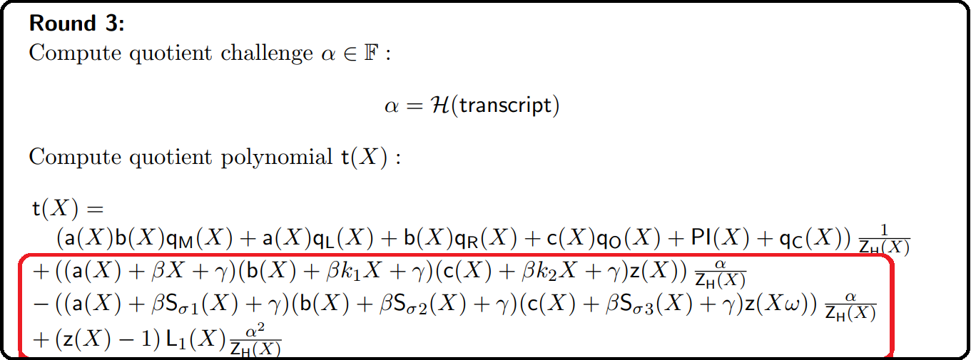
a) $L_1$ is $1$ at $a=1$ & $0$ at all other members of $H$ (by definition of the Lagrange Base). If at $a=\omega$, if $L_1(a)(z(a) - 1) = 0$, then it means $z(\omega) = 1$ - which if true, proves the first condition we are looking to prove.

b) As we go through 6(b) for each element $\in H$, it shows that $z$ has been built up accumulatively - i.e., each $z$ is the previous $z$ multiplied by the previous $m$.

So, proving 6a & 6b would prove our Copy Constraints.

In the $\mathcal{P} \mathfrak{lon}\mathcal{K}$ paper, this is done in Round 3 (Page 29).

Let’s go over only the part marked in red (the others are not part of the permutation check).

The last part of the red box is

$(z(X) -1)L_1(X) \frac {\alpha^2}{z_H}$

Here $z_H$ is the vanishing polynomial i.e.

$z_H(X) = (X-1)(X-\omega)(X-\omega^2)(X-\omega^3),…,(X-\omega^{n-1})$

i.e., $z_H=0$ at every element of the set $H$ - it vanishes at every element of $H$. If a prover wants to prove that a polynomial is zero (vanishes) at every element in a set, she divides the polynomial by the vanishing polynomial for that set. Only if it divides without a remainder will the prover be able to provide a commitment to the quotient of the division. So, if the prover is able to provide a commitment to a polynomial divided by $z_H$ and is able to open the commitment successfully, then it means that polynomial is zero on every element of the set $H$.

So, if the prover is able to do this for $(z(X) -1)L_1(X) \frac {\alpha^2}{z_H}$ (we will discuss the $\alpha$ term separately), it means $(z(X) -1)L_1(X) = 0$ at all points of $H$ including at $\omega$. Which means $(z(\omega) -1) = 0$ (because $L_1(1) = 1$).

Which means $z(\omega) = 1$ which was one of the things ($6(a)$) the prover set out to prove.

Next, let’s look at first 2 polynomials inside the red box in the earlier screenshot.

If we compare it with $f’(X)$ & $g’(X)$ we defined earlier, then the 2 equations can be rewritten as

$+ (f’(X)z(X))\frac {\alpha}{z_H} $

$- (g’(X)z(X\omega))\frac {\alpha}{z_H}$

If we ignore the $\alpha$ & $z_H$ terms this is

$f’(X)z(X) - g’(X)z(X\omega)$

This is the $6(b)$ statement which the prover needs to prove. This is divided by $z_H$ for the same reason. If the provers sends a commitment to this & opens it successfully, then it means that this polynomial is zero at all points of $H$ - i.e, proof for $6(b)$. About the $\alpha$ terms in both, it is explained here. Instead proving multiple different polynomials are zero at $H$, $\mathcal{P} \mathfrak{lon}\mathcal{K}$ combines them as linearly independent terms, so it can be proven together for all those polynomials.

Round 2 Notes

Some notes about the construction of $z(X)$ which happens in Round 2 in the $\mathcal{P} \mathfrak{lon}\mathcal{K}$ Paper

Here is a screenshot of Round 2 from Page 28 of the paper

The formula for Lagrange Interpolation is

$z(X) = \sum_{i=0}^{n-1} L_i Y_i$

where $L_i(X)$ is the $i$th Lagrange base.

We have $z(\omega) = 1$

i.e., for $X=\omega$, $Y=1$

$\omega$ is the 2nd element of $H$, so $Y_1 = 1$.

We can rewrite the Lagrange interpolation as

$z(X) = L_0 Y_0 + L_1 + \sum_{i=2}^{n-1} L_i Y_i$

Again, since the last+1 element is the first element (i.e., $n$ is same as index $0$ in the subgroup), we rewrite this as

$z(X) = L_1 + \sum_{i=2}^{n} L_i Y_i$

Also, we change the $\sum$ range by using $L_{i+1}$ instead of $L_i$

$z(X) = L_1 + \sum_{i=1}^{n-1} L_{i+1} Y_{i+1}$

So that’s what is used in the screenshot above. $Y_i$ is replaced by the equation to calculate $Y_i$. The numerator of the equation is the same as the $f’(X)$ we defined earlier & the denominator is $g’(X)$

Also, the term $(b_7 X^2 + b_8 X + b_9)z_H(X)$ is added while computing $z(X)$ for blinding which is explained here

Thus, we interpolate & compute the Permutation Polynomial $z(X)$. This polynomial is then used in Round 3 as discussed earlier to create a proof for the Copy Constraints.

Multiplicative Subgroup

Q: Why does $\mathcal{P} \mathfrak{lon}\mathcal{K}$ use a multiplicative subgroup?

A: There are multiple reasons why $\mathcal{P} \mathfrak{lon}\mathcal{K}$ uses a multiplicative subgroup

$(1)\space$ Every element of a finite field is a root of unity. A Finite Field $\mathbb F_p$ has a multiplicative subgroup of order $n$ only if $n$ divides $p-1$. All primitive roots of unity in a finite field also form a multiplicative subgroup of the field. Let $\omega$ be a primitive $n$th root of unity in $\mathbb F_p$ i.e. $\omega^n = 1$ This forms a multiplicative subgroup of order $n$ - let’s call it $H$

$H = \lbrace 1, \omega, \omega^2, \omega^3, …, \omega^{n-1} \rbrace$

This can support a circuit with a maximum of n gates.

In Groth16 with $n$ gates, we use $\lbrace 1, 2, 3, …, n \rbrace$ to represent the gates. There, we compute the vanishing polynomial as

$z_H(X) = (X-1)\cdot (X-2)\cdot(X-3) \dots \dots(X-n)$ (where 1, 2, 3 etc are the gate numbers)

The number of gates is usually very large (may be a million gates or more). So, computing the vanishing polynomial which has a million such terms is quite expensive.

$\mathcal{P} \mathfrak{lon}\mathcal{K}$ numbers the gates using the elements of the multiplicative subgroup $H$. Now the vanishing polynomial becomes

$z_H(X) = (X-1) \cdot(X-\omega)\cdot (X-\omega^2)\cdot …\cdot (X-\omega^{n-1})$

Now,

Let’s consider the polynomial $X^n - 1$

• For $X = 1$,

  $1^n = 1$, so $(X-1)$ is a root of $X^n - 1$

• For $X = \omega$,

  Since $\omega$ is the $n$th root of unity, $X^n = 1$ & hence $\omega$ is a root of $X^n - 1$

• For $X = \omega^2$

  ${\omega^2}^n = {\omega^n}^2 = {1}^2 = 1$.

  So $\omega^2$ is also a root of $X^n - 1$

• Like this, we can prove that every element of $H$ is a root of $X^n - 1$ & since $X^n - 1$ is degree $n$, the maximum number of roots it can have is $n$.

So $X^n - 1 = (X-1) \cdot (X-\omega)\cdot (X-\omega^2) \dots \dots (X-\omega^{n-1})$

So $z_H = X^n - 1$

So now the vanishing polynomial $Z_H$ is very easy to compute instead of having to multiply a million terms.

$(2)$ Using a multiplicative subgroup allows an efficient & elegant Product Check on the subgroup.

Take a look at $\mathcal{P} \mathfrak{lon}\mathcal{K}$’s Permutation proof.

This proof uses

$z(\omega X) = z(X) \cdot m(X) \qquad\qquad$ (where $m(X) = \frac {f’(X)}{g’(X)})$

We can define $z$ so because we are operating in a multiplicative subgroup $H = \lbrace 1,\omega, \omega^2, \omega^3, …, \omega^{n-1} \rbrace$, where multiplying by each element $\omega$ gives us the next element & thus we get the “right shift” relation between $z$ at an element & $z$ at the next element.

$(3)$ Using a multiplicative subgroup of a Finite Field is required for usage of Fast Fourier Transform to speed up some operations.

Blinding

Q: In Round 1 (Page 28 of the $\mathcal{P} \mathfrak{lon}\mathcal{K}$ paper), random blinding scalars are used to modify the 3 wire polynomials (the polynomials representing the left, right & output of the gates). What exactly is blinding?

A: Let’s say you have a polynomial $f(X)$ of degree $d$ & it’s commitment $C_f$. Let’s say the verifier selects random value $r$ & the prover sends the evaluation of $f$ at $r$ i.e. $f(r) = z$

A polynomial of degree $d$ can be recreated with $d+1$ evaluations by using Lagrange Interpolation. So, each opening of a Polynomial Commitment leaks some info about the polynomial.

Hence SNARKs use a trick called blinding to make it zero knowledge. Multiply the vanishing polynomial $z_H$ by a random Polynomial $R(X)$ & add it to $f(X)$ to create a new polynomial $F(X)$

$F(X) = R(X)\cdot z_H + f(X)$

Instead of committing and opening $f(X)$, the prover commits & opens $F(X)$.

$z_H$ is zero on the set the constraints are checked on - so on this set $F(X) = f(X)$. So other than in the commitment & opening, the SNARK can continue to use $f$ instead of $F$

The next question is what should be the degree of the random polynomial $R$. That depends on how many points you open $f$ at - if there is an opening at only one point, then $R$ needs to be of minimum degree $1$, if there are two openings, then there $R$ needs to be at least of degree $2$. The new polynomial $F(X)$ which is going to be opened instead of $f(X)$ has to be of degree of $f$ plus the number of points at which $f$ needs to be opened.

In Round 1, the left, right & output polynomials are evaluated only at one point each & hence a random polynomial of degree $1$ is used for blinding - for e.g. for blinding the opening of $a(X)$, $R(X) = (b_1 X + b_2)$ is used as the random polynomial. The round 2 polynomial $z(X)$ is evaluated at 2 points & hence a degree 2 random polynomial $(b_7 X + b_8 X + b_9)$ is used.

Linear Independence

Q: In Round 3 (Page 29), when combining different polynomials to form $t(X)$, why are different powers of $\alpha$ i.e. $ \alpha^0, \alpha^1, \alpha^2$ used.

A: Let’s say we have 4 polynomials - $f_1$, $f_2$, $f_3$ & $f_4 \in \mathbb F_p[X]$ where the max degree of these polynomials is $d$ which is very, very small as compared to $p$.

We want to combine them into one polynomial $f$ such that if $f$ is 0 at some point, then all of $f_i$’s are also zero at the same point.

Consider the set ${1, z, z^2, z^3}$ This is a linearly independent set.

We can use this set to combine four variables $a_1, a_2, a_3$ & $a_4$ like this

$g(Z) = a1 + a2\cdot Z + a3\cdot Z^2 + a4\cdot Z^3$

If $g(Z)=0$ at some $Z \ne 0$, then it means $a_1 = a_2 = a_3 = a_4 = 0$ (by the definition of a linearly independent set)

So, we can combine the polynomials $f_i$’s as

$f(X,Z) = f1(Z) + Z\cdot f2(x) + Z^2 \cdot f3(X) + Z^3\cdot f4(X)$

At some $X = r_1$, let

$f_1(r_1) = a_1$, $f_2(r_1) = a_2$, $f_3(r_1) = a_3$, $f_4(r_1) = a_4$,

So now

$f(X=r_1, X) = a1 + a2\cdot Z + a3\cdot Z^2 + a4\cdot Z^3$

At some random value $r_2$ chosen from $\mathbb F_p$, if

$f(X=r_1, Z = r_2) = 0$

then it means $a1 = a2 = a3 = a4 = 0$

i.e. $f_1(r_1, r_2) =f_2(r_1, r_2) = f_3(r_1, r_2) = f_4(r_1, r_2) = 0$

If $f_1$, $f_2$, $f_3$, $f_4$ are all $0$ at some random value $r_2$, then by the Schwartz-Zippel lemma, $f_1$, $f_2$, $f_3$, $f_4$ are all zero polynomials with very high probability because the maximum degree of these polynomials is very, very small as compared to $p$

So if we want to test if multiple polynomials are zero polynomials or not, we combine them using a lineraly independent set so we can test them with just one evaluation at a random point rather than testing them separately. Round 3 in the $\mathcal{P} \mathfrak{lon}\mathcal{K}$ paper creates the polynomial $t(X)$ with the linearly independent set $[1, \alpha, \alpha^2]$ to do this. In Round 5, the set $\lbrace 1, v, v^2, v^3, v^4, v^5 \rbrace$ is used to combine several polynomials to form a single opening proof polynomial $W_\zeta(X)$. It may be used at other places also.

Split Polynomials

Q: Why does the $\mathcal{P} \mathfrak{lon}\mathcal{K}$ protocol split the Quotient Polynomial into 3 polynomials?

A: In Round 3 (Page 29 of the $\mathcal{P} \mathfrak{lon}\mathcal{K}$ Paper), the Quotient Polynomial $t(X)$ is split into 3 polynomials

$t(X) = t’_{lo}(X) + X^n t’_{mid}(X) + X^{2n}t’_{hi}(X)$

This means 3 commitments are needed instead of one which increases proof size, so why is it done?

The tradeoff is that opening time gets reduced because of having smaller polynomials & hence the prover time gets reduced.

The opening time of a polynomial depends on the degree of the polynomial. However, having smaller polynomials may not help if the 3 polynomials are opened separately . The $\mathcal{P} \mathfrak{lon}\mathcal{K}$ paper presents a technique for batched opening of different polynomials at different points (on Page 10) which ensures that the opening time of 3 smaller polynomis is much lower than the opening time of one polynomial of roughly 3 times the size.

Field Element Reduction Optimisation

Q: In Round 5 (Page 30), the Linearisation Polynomial $r(X)$ is computed. What exactly is the Linearisation Polynomial?

A: Let’s look at how one proves the identity $h_1(X)\cdot h_2(X) - h_3(X) = 0$?

The normal way would be for the prover to send commitments for $h_1, h_2, h_3$. Then the verifier chooses a random number $r$ & the prover sends evaluation proofs for the 3 polynomials at $r$. The verifier then checks if $h_1(r)\cdot h_2(r) - h_3(r) \stackrel {?}{=} 0$.

$\mathcal{P} \mathfrak{lon}\mathcal{K}$ uses an optimisation which allows it to send one less evaluation proof.

This optimisation is based on the fact that Polynomial commitments like KZG are additively homomorphic, but not multiplicatively homomorphic.

$F(X) = f_0 + f_1X + f_2X^2 + … + f_dX^d$

$G(X) = g_0 + g_1X + g_2X^2 + … + g_dX^d$

Commitment Reference String = $\lbrace G, aG,a^2G, a^3G, …, a^dG \rbrace$

Commitment of $F$ & $G$ would be

$C_{F} = F(a)\cdot G = (f_0 + f_1a + f_2a^2 + … + f_da^d)\cdot G$

$C_{F} = f_0\cdot G + f_1a\cdot G + f_2a^2\cdot G + … + f_da^d\cdot G$

and

$C_{G} = g_0\cdot G + g_1a\cdot G + g_2a^2\cdot G + … + g_da^d\cdot G$

Now if we have a polynomial

$E(X) = F(X) + G(X) = f_0 + f_1X + f_2X^2 + … + f_dX^d + g_0 + g_1X + g_2X^2 + … + g_dX^d$

It’s obvious that the commitment for $E$ would be the sum of the commitments for $F$ & $G$

i.e. $C_{E} = C_F + C_G$

However the commitment is not multiplicatively homomorphic, i.e. if $H(X) = F(X) \cdot G(X)$, then you wouldn’t be able to compute the commitment of $H$ from those of $F$ & $G$.

Getting back to how the prover proves the identity $h_1(X)\cdot h_2(X) - h_3(X) = 0$

The prover evaluates $h_1$ at $r$ as $h_1(r) = c$ & sends the evaluation proof for the same. The verifier creates a new polynomial called as the Linearisation Polynomial

$L(X) = c\cdot h_2(X) - h_3(X)$

Because $h_1$ has been replaced by a constant $c$ in $L(X)$, $L$ doesn’t contains a multiplication of two polynomials. Hence the verifier can compute the commitment of $L$ by himself as

$C_L = c\cdot C_{h_2} - C_{h_3}$

where $C_L$, $C_{h_2}$ & $C_{h_3}$ are commitments of $L$, $h_2$ & $h_3$ respectively.

Since the commitment to $L$ has been computed using comittments to $h_2$ & $h_3$, verifying if $L(r) =0$ & $h_1(r) = c$ would be enough for the verifier to verify that $h_1(r)\cdot h_2(r) - h_3(r) {=} 0$. The verifier doesnt need to know the evaluation of $h_2$ & $h_3$ & prover doesn’t need to send the evaluation proofs for $h_2$ & $h_3$.

So instead of sending commitments to $h_1, h_2, h_3$ & evaluation proofs for all 3, the prover needs to send only commitments to $h_1, h_2, h_3$ & evaluation proofs for $L$ & $h_1$.

(In the $\mathcal{P} \mathfrak{lon}\mathcal{K}$ paper, this is on Page 18 titled “Reducing the number of field elements”).

The Prover wants to prove to the Verifier that she knows the solution to a particular equation without revealing the solution itself. In order for her to do this, in the Pinnochio & Groth16 zkSNARKs, she has to first transform the equation into the QAP (Quadratic Arithmetic Program) form. This post explains only the conversion part of these zkSNARKs.

This post is based on Vitalik Buterin’s write up on the same topic (with a partially similar title) but with some changes.

• In his write up, he doesn’t operate in a finite field though in the real world all these operations are done in a finite field. I think he has avoided finite fields to simplify the write up. However, I think not using finite fields ends up complicating it instead of simplifying it. His examples end up with scary looking floating point numbers. Working a finite field avoids this. Also since floating point operations are not precise, his final $T/Z$ polynomial division which should have no remainder ends up with an infinitesimal remainder if you try it out yourself. We will work in a finite field, $\mathbb F_p = GF(641)$.

• In the R1CS to QAP part of the transformation & beyond, I have shown the implementation using sagemath.

The equation

$x^3 + x + 5 = 35$ is the cubic equation the Prover knows the solution to & she has to convince the Verifier about this without revealing the solution to him. The solution is $x=3$

If you were to write a program in Python which takes a value for $x$ & evaluates the computation part of this equation, it would look something like this

def Evaluate(x):
    return x**3 + x + 5

Code Flattening

We first decompose the above code into a series of much simpler operations. This step is called flattening. In the flattened code, we are allowed only the following operations

• Assignment i.e. $x = y$, where $x$ is be a variable and $y$ can be a variable or a constant
• Operations like $x = y$ (Operator) $z$, where $x$ is a variable and $y$ and $z$ can be variables or constants. The only operators allowed are $+, -, *, /$

There is no return statement in the flattened code. Instead, we assign the return value to a variable “out”.

The flattened code

def Evaluate(x):
    var1 = x * x 
    var2 = var1 * x 
    var3 = var2 + x
    out  = var3 + 5

Conversion to Arithmetic Circuits & then R1CS

Next, we draw an arithmetic circuit of the above flattened program.

As we see from the circuit diagram, the circuit has 4 gates representing multiplication & addition operations & also has 5 variables & a constant $5$.

Let’s represent the variables in a solution vector $S$ (also called as witness)

$S = [1, out, x, var1, var2, var3]$

$1$ is included as an element of the vector so as to represent constants. For e.g. if we need a constant $5$, it will be represented as $5 * 1$

We now convert the Arithmetic Circuit into a Rank-1 Constraint System (R1CS). A R1CS is a triple of vectors $(l, r, o)$, and a solution vector $S$, such that $(l\cdot S) * (r\cdot S) = (o\cdot S)$ where $(\cdot)$ is the dot-product. Here $l$ stands for left (or left hand side of the multiplication) & $r$ for right of the multiplication & $o$ for output of each gate. We will have one triplet/constraint for each of the arithmetic gates.

Gate 1

Now in the circuit diagram, let’s take the first gate which represents $var1 = x * x$

For the purpose of the conversion, we look at it as $x * x = var1$. We now represent it as 3 vectors $l, r, o$. $l$ & $r$ is the vector on the left & right of the gate & $o$ is the output vector.

$l = [0, 0, 1, 0, 0, 0]$ (This represents the term $x$ which is to the left of the multiplication gate. Every element of the $l$ vector is 0 except the element corresponding to $x$ which has the value 1)

$r = [0, 0, 1, 0, 0, 0]$ (This represents the term $x$ which is to the right of the multiplication gate. Every element of the $r$ vector is 0 except the element corresponding to $x$ which has the value 1)

$o = [0, 0, 0, 1, 0, 0]$ (This represents $var1$ which is the output of the multiplication gate. Every element of the $o$ vector is 0 except the one corresponding to $var1$ which has the value 1)

Any solution vector which is correct will satify $(l.S) * (r\cdot S) = (o\cdot S)$.

Let us try this out. We know the solution of the equation $x^3 + x + 5 == 35$ is $x = 3$. So substitute our solution vector $S = [1, out, x, var1, var2, var3]$ with the actual values based on $x = 3$

$var1 = x * x = 3 * 3 = 9$

$var2 = var1 * x = 9 * 3 = 27$

$var3 = var2 + x = 27 + 3 = 30$

$out = var3 + 5 = 30 + 5 = 35$

So $S = [1, 35, 3, 9, 27, 30]$

Dot product of any two vectors $p = [p_1, p_2, …, p_n]$ and $q = [q_1, q_2, …, q_n]$ is defined as

$p \cdot q = \sum_{i=1}^{n} = {p_1}{q_1} + {p_2}{q_2} + … + {p_n}{q_n}$

So $l\cdot S = [0, 0, 1, 0, 0, 0]\cdot[1, 35, 3, 9, 27, 30]$

$l\cdot S = 0 * 1 + 0 * 35 + 1 * 3 + 0 * 9 + 0 * 27 + 0 * 30 = 3$

Likewise $r.S = 3$ and $o.S = 9$

So $(l\cdot S) * (r\cdot S) = 3 * 3 = 9 = (o\cdot S)$.

So $(l\cdot S) * (r\cdot S) = (o\cdot S)$ is satisfied - this is a satisfied R1CS - it shows that the solution vector satisfies Gate 1

Gate 2

Let’s take the 2nd gate which represents $var1 * x = var2$

$l = [0, 0, 0, 1, 0, 0]$ (This represents the term $var1$ which is to the left of the multiplication gate. Every element of the $l$ vector is 0 except the element corresponding to $var1$ which has the value 1)

$r = [0, 0, 1, 0, 0, 0]$ (This represents the term $x$ which is to the right of the multiplication gate. Every element of the $r$ vector is 0 except the element corresponding to $x$ which has the value 1)

$o = [0, 0, 0, 0, 1, 0]$ (This represents the term $var2$ which is the output of the multiplication gate. Every element of the $o$ vector is 0 except the element corresponding to $var2$ which has the value 1)

Gate 3

3rd gate is the addition gate which represents $var2 + x = var3$. The vectors for addition gates are derived differently. The equation is equivalent to $(var2 + x) * 1 = var3$. So the $l$ vector represents $var2 + x$, the $r$ vector represents $1$ & the $o$ vector represents $var3$

$l = [0, 0, 1, 0, 1, 0]$ (This represents $var2 + x$)

$r = [1, 0, 0, 0, 0, 0]$ (This represents $1$)

$o = [0, 0, 0, 0, 0, 1]$ (This represents $var3$)

Gate 4

Likewise, the 4th gate $var3 + 5 = out$ is equivalent to $(var3 + 5) * 1 = out$

$l = [5, 0, 0, 0, 0, 1]$ ($var3 + 5$)

$r = [1, 0, 0, 0, 0, 0]$ ($1$)

$o = [0, 1, 0, 0, 0, 0]$ ($out$)

Though we aren’t explicitly calculating & showing it here, $(l\cdot S) * (r\cdot S) = (o\cdot S)$ is satisfied for Gates 2, 3 & 4 also. We now have the complete R1CS with 4 constraints.

We can create a Matrix $L$ by using each of $l$ vectors as a row in the Matrix. Likewise Matrices $R$ & $O$.

The Complete Satisfied R1CS is

\(L = \begin{pmatrix} 0&0&1&0&0&0 \\ 0&0&0&1&0&0 \\ 0&0&1&0&1&0 \\ 5&0&0&0&0&1 \end{pmatrix}\) \(R = \begin{pmatrix} 0&0&1&0&0&0 \\ 0&0&1&0&0&0 \\ 1&0&0&0&0&0 \\ 1&0&0&0&0&0 \\ \end{pmatrix}\) \(O = \begin{pmatrix} 0&0&0&1&0&0 \\ 0&0&0&0&1&0 \\ 0&0&0&0&0&1 \\ 0&1&0&0&0&0 \\ \end{pmatrix}\)

This along with our solution vector $S = [1, out, x, var1, var2, var3]$ forms our R1CS.

Let’s define these matrices in sage. I have shown only 1 below, but the remaining 2 will also be defined similarly.

p = 641
Fp = GF(p)
Rng.<x> = PolynomialRing(Fp)

L = Matrix(Fp, [
    [0,0,1,0,0,0],
    [0,0,0,1,0,0],
    [0,0,1,0,1,0],
    [5,0,0,0,0,1]]
    )

QAP

The next step is taking this R1CS and converting it into the QAP form, which implements the exact same logic except using polynomials. In the construction used, the number of polynomials & their degree would depend on the length of the solution vector & the number of gates. The solution vector contains 6 elements, so we can construct 6 polynomials. Each gate contributes 1 point to each polynomial. We have 4 gates here, we get 4 points per polynomial. 4 points allows us to define a polynomial of maximum degree 3. So we can construct 6 polynomials each with a maximum degree of 3. So we can transform our matrices collectively into 6 polynomials, each of degree 3.

A polynomial of degree $n$ is defined by a minimum of $n+1$ points. Each column of $L$, $R$ & $O$ has 4 elements. So each such column can be converted to a polynomial of degree 3. We use Lagrange’s Polynomial Interpolation to do this.

For e.g. 1st column of $L$ is $[0, 0, 0, 5]^T$ (shown transposed). We can consider each element as the y-coordinate corresponding to $x \in [1, 2, 3, 4]$. So we get $4$ sets of points - $(1,0), (2,0), (3,0), (4,5)$. This is an arbitrary interpretation which we use to convert the R1CS into the QAP form. We could have just as well used $[5, 7, 9, 11]$ instead of $[1, 2, 3, 4]$ as long as we are consistent across all equations..

We can find the polynomial passing through these 4 points using Lagrange Interpolation.

Rng.<x> = PolynomialRing(Fp) # Polynomial Ring in GF(641)
points = [(1,0), (2,0), (3,0), (4,5)]
Rng.lagrange_polynomial(points)
535*x^3 + 636*x^2 + 116*x + 636

So the polynomial corresponding to the first Column of $L$ is

$535x^3 + 636x^2 + 116x + 636$

Since we have $18$ polynomials to interpolate, we can do it in loops in sage. And after calling Rng.lagrange_polynomial(points), we call the coefficients method on the output polynomial (i.e. Rng.lagrange_polynomial(points).coefficients(sparse=False)) which transforms the coefficients of each output polynomial into a list which we then collect in a Matrix.

M = [L, R, O]
PolyM = []
for m in M:
    PolyList = []
    for i in range(m.ncols()):
        points = []
        for j in range(m.nrows()):
            points.append([j+1,m[j,i]])
        Poly = Rng.lagrange_polynomial(points).coefficients(sparse=False)
        if(len(Poly) < m.nrows()):
            # if degree of the polynomial is less than 4
            # we add zeroes to represent the missed out terms
            dif = m.nrows() - len(Poly)
            for c in range(dif):
                Poly.append(0);
        PolyList.append(Poly)
    PolyM.append(Matrix(Fp, PolyList))

If we print out the 3 matrices holding 6 polynomials each we get

# PolyM[0] = Lm (Matrix of L Polynomials) 
[636 116 636 535]
[  0   0   0   0]
[  8 416   5 213]
[635 330 637 321]
[  4 634 324 320]
[640 536 640 107]

# PolyM[1] = Rm (Matrix of R Polynomials)
[  3 529 323 427]
[  0   0   0   0]
[639 112 318 214]
[  0   0   0   0]
[  0   0   0   0]
[  0   0   0   0]

# PolyM[2] = Om (Matrix of O Polynomials)
[  0   0   0   0]
[640 536 640 107]
[  0   0   0   0]
[  4 423 322 534]
[635 330 637 321]
[  4 634 324 320]

For convenience, we will refer to $PolyM[0]$, $PolyM[1]$ & $PolyM[2]$ as $Lm$,$Rm$ & $Om$

You can see the polynomial we got from the first column of $L$ (i.e $535x^3 + 636x^2 + 116x + 636$) appear in first row here of the Matrix $Lm$ . The Row is to be interpreted in reverse order - i.e $[636\ 116\ 636\ 535]$ is $535x^3 + 636x^2 + 116x + 636$

This finishes the transformation of the problem to the QAP Form. What do we achieve by converting it into the QAP form? Instead of checking the constraints in the R1CS individually, we can now check all of the constraints at the same time by doing the dot product check on the polynomials.

Let’s take a closer look at $Lm$ \(\begin{pmatrix} 636&116&636&535 \\ 0&0&0&0 \\ 8&416&5&213 \\ 635&330&637&321 \\ 4&634&324&320 \\ 640&536&640&107 \end{pmatrix}\)

This has 6 left polynomials, one in each row.

Our solution vector $S = [1, out, x, var1, var2, var3]$ also has 6 elements. So we can do a dot product of $S\cdot Lm$ whose output again will be a polynomial. Likewise for the other 2 polynomial matrices.

# We define the solution vector also in the field
S = vector(Fp,[1, 35, 3, 9, 27, 30])

# Create the Lx, Rx & Ox polynomial
# In the program, we use Fx to denote F(x)
Lx = Rng(list(S*PolyM[0]))
Rx = Rng(list(S*PolyM[1]))
Ox = Rng(list(S*PolyM[2]))
print("Lx = " + str(Lx))
print("Rx = " + str(Rx))
print("Ox = " + str(Ox))

Lx = 529*x^3 + 359*x^2 + 354*x + 43
Rx = 428*x^3 + 636*x^2 + 224*x + 638
Ox = 537*x^3 + 296*x^2 + 499*x + 600

So by taking a dot product of $S$ with each of $Lm$, $Rm$ and $Om$, we created 3 polynomials $L(x)$, $R(x)$ and $O(x)$

We can define a new polynomial $T(x) = L(x) * R(x) - O(x)$.

....: # New Polynomial T
....: T = Lx*Rx - Ox
....: print("T(x) = ", end="")
....: print(T)
T(x) = T(x) = 139*x^6 + 372*x^5 + 275*x^4 + 58*x^3 + 147*x^2 + 379*x + 553

In the R1CS, we had checked if $(l\cdot S) * (r\cdot S) = (o\cdot S)$ for each of the Gates. After conversion to QAP, we can do the same by checking the value of $T$ at $x$ at $1, 2, 3, 4$ - if all 4 are zero, then we have checked all the constraints together - thereby proving that the solution vector known to the Provers satisfies the equation.

....: #Let's check Tx at x = 1, 2, 3, 4
....: print("T(1) = " + str(T(1)))
....: print("T(2) = " + str(T(2)))
....: print("T(3) = " + str(T(3)))
....: print("T(4) = " + str(T(4)))
....:
T(1) = 0
T(2) = 0
T(3) = 0
T(4) = 0

However, the Verifier doesn’t know the polynomial $T$, nor can he compute it since he doesn’t know the solution vector. So the Prover has to prove it to the Verifier that $T$ is zero at $x=1, x=2, x=3,x=4$. If $T$ is zero at $x=1, x=2, x=3,x=4$, then it means these are all roots of $T$. So we create a new polynomial $Z$ known by both the Prover & the Verifier.

$Z(x) = (x-1)(x-2)(x-3)(x-4)$

If $T$ is divided by $Z$, then it will be perfectly divisible & will leave no remainder i.e. there must exist a Polynomial $H$ such that $T(x) = H(x) \cdot Z(x)$

Let’s check this out in sagemath

Z = Rng((x-1)*(x-2)*(x-3)*(x-4))
H = T.quo_rem(Z)
print("Quotient of T/Z = ", end="")
print(H[0])
print("Remainder of T/Z = ", end="")
print(H[1])

Quotient of Z/T = 139*x^2 + 480*x + 210
Remainder of Z/T = 0

The reason we get a $0$ remainder is because $Z$ divides $T$. If you change even a single element in the solution vector, then $T$ will no longer divide $Z$ exactly & you will end up with a remainder.

In a typical zkSNARK, the prover proves that $Z$ exactly divides $T$ using Polynomial Commitments & Elliptic Curve Bilinear Pairings. You can take a look at my Groth16 post to check how it’s done in Groth16.

Note: An older version of this post used $\mathbb F_{41}$, it’s been updated to use $\mathbb F_{641}$ now.

Introduction

Commitment schemes are fundamental components of many cryptographic protocols. A secure commitment scheme allows a committer to publish a value, called the commitment, which binds her to a message (binding) without revealing it (hiding). Later, she may open the commitment and reveal the committed message to a verifier, who can check that the message is consistent with the commitment.

Consider the following scenario.

• Peggy wants to commit to a message $m$. To do so, she writes down $m$ on a piece of paper, puts it in a box, and locks it using a padlock.

• Peggy gives the box to Victor.

• If Peggy wants to, she can later open the commitment by giving Victor the key to the padlock.

There are two basic properties here, which are essential to any commitment scheme:

• Having given away the box, Peggy cannot anymore change what is inside. Hence, when the box is opened, we know that what is revealed really was the choice that Peggy committed to originally. This is called the Binding property.

• When Victor receives the box, he cannot tell what is inside before Peggy decides to give him the key. This is called the Hiding property.

Polynomials are frequently used in cryptography because they can be used to encode a lot of information. A Polynomial Commitment Scheme (PCS) allows the committer to commit to a polynomial with a commitment string that can be used by a verifier to confirm claimed evaluations of the committed polynomial. We will look at one such PCS called KZG (Kate, Zaverucha, Goldberg). It’s also referred to as the Kate Commitment Scheme.

Pre-requisite topic before we discuss the KZG PCS

Elliptic Curve Pairings

An Elliptic Curve Pairing is defined as a map

$e : \mathbb G_1 \times \mathbb G_2 \mapsto \mathbb G_T$

$\mathbb G_1$ can be equal to $\mathbb G_2$ i.e. $\mathbb G_1 = \mathbb G_2 = \mathbb G$. Such a pairing is called as a Symmetric Pairing. If they are not equal, then it’s called as an Asymmetric Pairing.

Let $G_1$ & $G_2$ be generators of $\mathbb G_1$ & $\mathbb G_2$ respectively. Let $a$ & $b$ be scalars. The core property of Elliptic Curve Pairings which we use the most is the following.

$e(a G_1, b G_2) = e(b G_1, a G_2) = e(ab G_1, G_2) = e(G_1, ab G_2) = e(G_1, a G_2)^{b} = e(G_1, G_2)^{ab}$

If you are not familiar with pairings, I have given a small introduction to Pairings as part of this post - Weil Pairing and the MOV attack.

The Schwartz-Zippel Lemma

Let $f$ be a polynomial from $\mathbb F_p[x]$ of degree less than or equal to $d$. Let $p \approx 2^{256}$ & $d \le 2^{40}$. If we test $f$ at a random value $r \in \mathbb F_p$, then the probability that $f(r) = 0$ would be $\frac {d}{p}$ which for these values of $d$ & $p$ would be very, very small. So, if $f(r) = 0$, then with high probability, $f$ is a zero polynomial (i.e., zero at all points). This is a simple test to check if a committed polynomial is a zero polynomial. Open the commitment to the polynomial at a random point & if it opens to zero, then it is a zero polynomial.

This also helps to prove that 2 polynomials are equal. If the 2 polynomials are $f$ & $g$, we create a new polynomial $p(x) = f(x)\space - \space g(x)$.

If we test $p$ at a random $r \in \mathbb F_p$ & $f(r)$ turns out to be $0$, then $p$ is a zero polynomial with very high probability. If $p$ is a zero polynomial, then it obviously means $f = g$.

The Commitment Scheme tests the polynomials only at a small number of points ($a$ & the opening point). The Binding property of the commitment scheme is based on the Schwartz-Zippel Lemma.

The Commitment Scheme

Let $F(x)\in \mathbb F_p[x]$ be the polynomial which needs to be committed. $F(x)$ is a polynomial of degree $d$ or less.

We will first describe the commitment using Symmetric Elliptic Curve Pairing - i.e. $e : \mathbb G \times \mathbb G \mapsto \mathbb G_T$. $\mathbb G$ is an Elliptic Curve group of order $p$ with a generator $G$.

Trusted Setup

The first stage of the commitment scheme is a trusted setup. During the trusted setup, a random value $a \in \mathbb F_p$ is sampled. Then the following tuple of size $d+1$ known as the Reference String is generated - $\lbrace G, aG,a^2G, a^3G, …, a^dG \rbrace$. After generating the tuple, the random value $a$ is destroyed such that it’s not known to anyone including the Prover or the Verifier. The destroyed value is called as toxic waste. If toxic waste is known to anyone, they can use it to generate fraud proofs.

Commitment

Let’s denote the commitment of the polynomial $F(x)$ as $C_F$ where

$C_F = F(a)\cdot G$ where $F(a)$ is the polynomial evaluated at $x=a$.

Though $a$ has been deleted, the committer can stil compute the commitment using the Reference String.

Let $F(x) = f_0 + f_1x + f_2x^2 + … + f_dx^d$

$F(a) = f_0 + f_1a + f_2a^2 + … + f_da^d$

So $C_F = F(a)\cdot G = (f_0 + f_1a + f_2a^2 + … + f_da^d)\cdot G$

$C_F = f_0\cdot G + f_1a\cdot G + f_2a^2\cdot G + … + f_da^d\cdot G$

Though the committer doesn’t know $a$, she knows $\lbrace G, aG,a^2G, a^3G, …, a^dG \rbrace$ from the reference string & can evaluate $C_F$ & evaluate the commitment. The committer sends the commitment to the verifier.

Since $G$ is a generator of the Elliptic Curve group $\mathbb G$, the commitment is a point on the Elliptic Curve.

The Hiding property of the commitment is based on the Discrete Logarithm problem being hard in $\mathbb G$

Full Open & Verify

In a full open, the committer sends the polynomial to the verifier & the verifier can use the reference string & compute the commitment himself & verify if it matches with the commitment sent originally by the committer.

Partial Open or Evaluation Proof

In KZG, committer can also do a partial open (i.e. evaluation at a single value) which is called as the Evaluation Proof.

The verifier sends a value $b$ randomly selected from $\mathbb F_p$ to the committer. The committer evaluates the polynomial $F(x)$ at $x=b$ as $F(b) = c$ & sends $c$ to the verifier. The committer also has to provide a proof to the verifier that $F(b) = c$.

The proof which the committer provides to the verifier is the commitment of the Quotient Polynomial $Q(x)$ i.e. $C_Q$

$Q(x)$ is defined as

$Q(x) = \frac {F(x) - F(b)} {x-b} = \frac {F(x) - c} {x-b}$

As per Little Bezout’s Theorem, if $F(x)$ is a polynomial, then $F(x) - F(b)$ is perfectly divisible by $(x-b)$ i.e. the remainder is $0$. So $Q(x)$ above is a polynomial i.e. it won’t have any variable in the denominator or any negative exponents. Since $Q(x)$ is a polynomial, then the committer can calculate the commitment of $Q(x)$ using the Reference String as

$C_Q = Q(a)\cdot G$

If $F(x)$ weren’t perfectly divisible by $(x-b)$, then $Q(x)$ would have a denominator & negative exponents & the commiter wouldn’t be able to evaluate it using just the Reference String & without knowing $a$.

The committer sends $C_Q$ to the verifier as the Evaluation Proof.

Verifying

A commitment scheme is said to be complete if anything which is true is provable. It is said to be sound if everything which is provable is true - i.e. anything which is false cannot be proven by the scheme.

The verifier has $C_F$, $C_Q$ & $c$. He needs to verify that $F(b) = c$

$Q(x) = \frac {F(x) - c} {x-b}$

So,

$(x-b)\cdot Q(x) = F(x) - c$

If you evaluate this at $x = a$, it becomes

$(a-b)\cdot Q(a) = F(a) - c$

Multiplying both sides by the generator $G$, we get

$(a-b)\cdot Q(a)\cdot G = F(a)\cdot G - c\cdot G$

Now, $C_Q = Q(a)\cdot G$ & $C_F = F(a)\cdot G$. So substituting, we get

$(a-b)\cdot C_Q = C_F - c\cdot G$

If the verifier is able to verify that the above equality holds good, then he has verified the commitment. But since the verifier doesn’t know the value of $a$, he cannot directly verify if this equality holds good.

However, the verifier can use Elliptic Curve Pairings to verify whether the above equality holds even without knowing $a$. The pairing is denoted by the map

$e:\space \mathbb G$ X $\mathbb G \mapsto \mathbb G_T$

This is the equality to check

$(a-b)\cdot C_Q \stackrel {?}{=} C_F - c\cdot G$

Each input to the pairing map needs to be an element of the Group. Any commitment is a scalar multiple of the generator of the group, so both $C_F$ & $C_Q$ are elements of $\mathbb G$. Since $C_Q$ is an element of the group, multiplying it with the scalar $a-b$ also will result in an element of the group. So $(a-b)\cdot C_Q$ is also an element of $\mathbb G$. $C_F$ & $c\cdot G$ are both elements of the group, so $C_F - c\cdot G$ is also an element of the group. So all the terms in the equality are group elements. So they can be inputs to the pairing map.

By passing the sides of the equality as the first parameter to the map & pass $G$ as the 2nd param for each side, we can turn the equality to be verified into

$e((a-b)\cdot C_Q, G) \stackrel {?}{=} e(C_F - c\cdot G, G)$

This still doesn’t help us because we don’t know $a$.

However, bilinearity property of the pairing map means that

$e(\alpha A,B) = e(A, \alpha B)$ if $\alpha$ is a scalar.

So we can rewrite it as

$e(C_Q, (a-b)\cdot G) \stackrel {?}{=} e(C_F - c\cdot G, G)$

Further simplifying

$e(C_Q, aG - bG) \stackrel {?}{=} e(C_F - cG, G)$

Though we don’t know $a$, we do know $aG$ from our Reference String. So now the verifier can check whether the above equality is true or not. This ends the proof.

Note that any pairing based equality check $e(A, B) \stackrel {?}{=} e(P,Q)$ can also be expressed in a diff way.

$e(A, B) \stackrel {?}{=} e(P,Q)$

$e(A, B) \stackrel {?}{=} e((-1)\cdot (-P),Q)$

Again using the bilinearly property on the Right hand side, we get

$e(A, B) \stackrel {?}{=} e(-P,Q)^{-1}$

which is the same as

$e(A, B)\cdot e(-P,Q) \stackrel {?}{=} 1$

Many texts & papers represent pairing based checks in the above way.

Asymmetric Pairings

Above, we used a symmetric pairing to prove the correctness of the above verification equation. However, an Asymmetric Pairing (i.e. $\mathbb G_1 \ne \mathbb G_2$) can also be used & is usually preferred. The proof for the verify equation using Asymmetric Pairings is very similar & given below.

Let’s start from this point in the earlier proof.

$(a-b)\cdot Q(a) \stackrel {?}{=} F(a) - c$

Multiplying both sides by $G_1$

$(a-b)\cdot Q(a)\cdot G_1 \stackrel {?}{=} F(a) \cdot G_1 - c \cdot G_1$

$(a-b)\cdot C_Q \stackrel {?}{=} C_F - c \cdot G_1$

Using pairings,

$e((a-b)\cdot C_Q,G_2) \stackrel {?}{=} e(C_F - c \cdot G_1, G_2)$

Using the bilinear property,

$e(C_Q,(a-b)\cdot G_2) \stackrel {?}{=} e(C_F - c \cdot G_1, G_2)$

$e(C_Q,a\cdot G_2 - b\cdot G_2) \stackrel {?}{=} e(C_F - c \cdot G_1, G_2)$

Everything except $a\cdot G_2$ is either calculated or found in the SRS for $G_1$. And $a\cdot G_2$ will be part of the SRS for $G_2$ & that is also known and thus the equality can be verified.

Batch Mode

Batch Mode Single Polynomial, multiple points

KZG commitments can also be opened & verified at multiple points using a single proof.

In the stand-alone opening, the committer evaluated $F(x)$ at $b \in \mathbb F_p$ as $F(b) = c$ & provided $c$ along with the proof to the verifier.

In batch mode, the verifier sends to the committer a set of values $ B = \lbrace b_1, b_2, b_3, …, b_t \rbrace$ such that $t \lt d$, the committer evaluates $f(b_1) = c_1, f(b_2) = c_2, …, f(b_t) = c_t$ and constructs the set $C = \lbrace c_1, c_2, c_3, …, c_t \rbrace$.

Let $P(x) = (x-b_1)(x-b_2)…(x-b_t)$

Since the degree of $F(x)$ is $d$ & $t \lt d$, we can divide $F(x)$ by $P(x)$. Let the quotient of the division be $Q(x)$ & the remainder be $R(x)$ (Note that we aren’t saying here that $F(x)$ is divisible by $Q(x)$, so we have remainder here).

i.e. $F(x) = P(x) Q(x) + R(x)$

The committer computes $Q(x)$ & also the commitment for $Q(x)$ i.e. $C_Q$ & sends those also to the verifier along with the set $C$

The committer can also send $R(x)$ to the verifier. Alternately, the verifier can also find the polynomial $R(x)$ himself as shown below.

$F(x) = P(x) Q(x) + R(x)$ with $P(x) = (x-b_1)(x-b_2)…(x-b_t)$

For any $b_i \in B = \lbrace b_1, b_2, b_3, …, b_t \rbrace$, it’s pretty apparent that $P(x)$ is zero. & hence the middle term vanishes at all $b_i \in B$.

So for all $b_i \in B$, $F(x) = R(x)$

Since $F(b_i) = c_i$ for all $\lbrace b_i \in B, c_i \in C \rbrace$, likewise

$R(b_i) = c_i$ for all $\lbrace b_i \in B, c_i \in C \rbrace$

Since the degree of $Q(x)$ is $t$ & $R(x)$ is the remainder of dividing $F(x)$ by $Q(x)$, the degree of $R(x)$ is less than $t$. Since the verifier knows evaluation of $R(x)$ at $t$ points, he can find $R(x)$ using Lagrange’s Interpolation. So now $R(x)$ is known to the verifier.

The Verifier can also find the polynomial $P(x)$ which is

$P(x) = (x-b_1)(x-b_2)…(x-b_t)$

The Verifier also computes the commitments of $P(x)$ & $R(x)$

$C_P = P(a)\cdot G$

$C_R = R(a)\cdot G$

Now the verifier can verify the Batch Evaluation by doing the following steps.

1) Verifier checks if $F(b_i) \stackrel {?}{=} R(b_i)$ for all $b_i \in B$. The committer has provided the set $C$ which are the evaluations of $F(x)$ at all $b_i \in B$. And the verifier knows $R(x)$, so he can also evaluate $R(x)$ at all the $b_i \in B$. So he can verify if $F(b_i) \stackrel {?}{=} R(b_i)$ for all $b_i \in B$

2) The verifier has to verify that the following equality holds

$F(x) \stackrel {?}{=} P(x) Q(x) + R(x)$

$F(x) - R(x) \stackrel {?}{=} P(x) Q(x)$

Multiply both sides by the generator $G$

$F(x)\cdot G - R(x)\cdot G \stackrel {?}{=} P(x) Q(x)\cdot G$

Evaluate the above at $a$

$F(a)\cdot G - R(a)\cdot G \stackrel {?}{=} P(a) Q(a)\cdot G$.

$F(a)\cdot G$ is the committment of $F$ i.e. $C_F$. Likewise, 2 other terms above are also committments. So,

$C_F - C_R \stackrel {?}{=} P(a)\cdot C_Q$

The verifier needs to evaluate the above to verify the proof. However, since $a$ is unknown, he cannot evaluate $P(a)$. But like before, he can use pairings.

$C_F$ & $C_R$ are both elements of $\mathbb G$, so $C_F - C_R$ is also an element of $\mathbb G$

$C_Q$ is an element of $\mathbb G$ & $P(a)$ is a scalar. So $P(a)\cdot C_Q$ is also an element of $\mathbb G$.

So we can apply the pairing map to both sides

$e(C_F - C_R, G) \stackrel {?}{=} e(P(a)\cdot C_Q, G)$

Note that $P(a)$ is a scalar here.And the bilinearity property of the pairing map means that

$e(\alpha A,B) = e(A, \alpha B)$ where $\alpha$ is a scalar.

So, we can rewrite the Right Hand Side as

$e(C_F - C_R, G) \stackrel {?}{=} e(C_Q, P(a)\cdot G)$

$C_P= P(a).G$, so

$e(C_F - C_R, G) \stackrel {?}{=} e(C_Q, C_P)$

The verifier knows all the terms of this pairing & can evaluate to the check if the equality holds or not.

Batch Mode Multiple Polynomials, same point

Note: The KZG paper covers standalone openings & batch opening of a single polynomial at multiple points.

However, there are also protocols for batch opening of multiple polynomials at the same point & batch opening of multiple polynomials at multiple points. Both are covered in the PLONK paper. These protocols are described below.

Consider $f_1, f_2,…, f_t \in \mathbb F_p[x]$ with $t < d$ & $z\in \mathbb F_p$. Let $C_{f_1},C_{f_2}, …, C_{f_t}$ be the commitments to these polynomials.

The openings $f_1(z)=s_1, f_2(z) = s_2, … ,f_t(z)= s_t$ have to be verified.

• Verifier sends random $\gamma \in \mathbb F_p$ to Prover

• Prover computes the polynomial

$\qquad h(x) = \sum_{i=1}^t \gamma^{i-1} \cdot \frac {f_i(x) - f_i(z)}{x-z}$

• Prover computes & sends $C_h$, the commitment for $h(x)$ to the verifier.

Now,

$f_i(z) = s_i$

Verifier has to check if

$h(x) \stackrel {?}{=} \sum_{i=1}^t \gamma^{i-1} \cdot \frac {f_i(x) - s_i}{x-z}$

$h(x)(x-z) \stackrel {?}{=} \sum_{i=1}^t \gamma^{i-1} \cdot (f_i(x) - s_i)$

$h(x)(x-z) \stackrel {?}{=} \sum_{i=1}^t \gamma^{i-1} \cdot f_i(x) - \sum_{i=1}^t \gamma^{i-1} \cdot s_i$

Multiplying both sides by G & evaluating at $x=a$

$h(a)\cdot G \cdot (a-z) \stackrel {?}{=} \sum_{i=1}^t \gamma^{i-1} \cdot f_i(a)\cdot G - \sum_{i=1}^t \gamma^{i-1} \cdot s_i\cdot G $

$C_h = h(a)\cdot G$

$C_{f_i} = f_i(a)\cdot G$

$C_h \cdot (a-z) \stackrel {?}{=} \sum_{i=1}^t \gamma^{i-1} \cdot C_{f_i} - \sum_{i=1}^t \gamma^{i-1} \cdot s_i\cdot G \quad — (Eq\space\space 1)$

Let $F = \sum_{i=1}^t \gamma^{i-1} \cdot C_{f_i}$

Let $v = \sum_{i=1}^t \gamma^{i-1} \cdot s_i\cdot G$

Substituting the above in $(Eq\space\space 1)$

$C_f \cdot (a-z) \stackrel {?}{=} F - v \quad — (Eq\space\space 2)$

Using pairings,

$e(C_f \cdot (a-z), G) \stackrel {?}{=} e(F - v, G)$

Using the bilinearity property,

$e(C_f, (a-z)\cdot G) \stackrel {?}{=} e(F - v, G)$

$e(C_f, aG - zG) \stackrel {?}{=} e(F - v, G)$

$z$ is known, so $zG$ is known. $aG$ is known from the SRS. $F$ & $v$ are also computable. So all the terms in the above are known & the verifier can check if the equality holds or not.

Batch Mode Multiple Polynomials, multiple points

In this case, we have $f_1, f_2,…, f_t \in \mathbb F_p[x]$ & $t < d$ with $z\in \mathbb F_p$. Let $C_{f_1},C_{f_2}, …, C_{f_t}$ be the commitments to these polynomials.

We also have $f’_1, f’_2,…, f’_t \in \mathbb F_p[x]$ with $t’ < d$ & $z’\in \mathbb F_p$.

Let $C_{f_1’},C_{f_2’}, …,C_{f_{t’}’}$

be the commitments to these polynomials.

And likewise $f’'_i$s, with $z’’$ and many more such sets.

Let’s, for a moment, assume we have only 2 such sets $f$ & $f’$ & batch them together. We can extend the same method for any number of such sets.

In the multiple polynomial, same point protocol, $F$ & $v$ were computed, now we also have $F’$ & $v’$. $F$ & $F’$ can be computed in parallel. And likewise $v$ & $v’$. So similar to $(Eq 2)$, we have

$C_f \cdot (a-z) \stackrel {?}{=} F - v$

$C_{f’} \cdot (a-z’) \stackrel {?}{=} F’ - v’$

Verifier sends a random $r \in \mathbb F_p$, and Prover uses it to combine the above 2 equatons in a linearly independent way so that they can be tested together. This trick is explained here.

$C_f(a-z) + r\cdot C_{f’}\cdot (a-z’) \stackrel {?}{=} F + rF’ - v - rv’$

Let $H = F+rF’ - v - rv’$

$C_f(a-z) + r\cdot C_{f’}\cdot (a-z’) \stackrel {?}{=} H$

$a \cdot C_f + ra \cdot C_{f’} \stackrel {?}{=} H + z\cdot C_f + z’r\cdot C_{f’}$

$a(C_f + r \cdot C_{f’}) \stackrel {?}{=} H + z\cdot C_f + z’r\cdot C_{f’}$

Using pairings,

$e(a(C_f + r \cdot C_{f’}), G) \stackrel {?}{=} e(H + z\cdot C_f + z’r\cdot C_{f’}, G)$

Using the bilinearity property

$e(C_f + r \cdot C_{f’}, aG) \stackrel {?}{=} e(H + z\cdot C_f + z’r\cdot C_{f’}, G)$

So all the terms in the above are known & the verifier can check if the equality holds or not.

For more than 2 sets, we will combine them linearly independent using $\lbrace 1, r, r^2, r^3, …\rbrace$ as explained.

One of the advantages of the KZG PCS is that the commitment size is constant. Irrespective of how long the polynomial is (i.e. degree of the polynomial), the commitment is always just one element of the group $\mathbb G$. Likewise, the evaluation proof is also a commitment, so there again, the size is constant for the evaluation proof both at a single value and also in batch mode.

Why Elliptic Curve Cryptography?

Q. Why does modern cryptography prefer the discrete log problem over the additive group of points on an Elliptic Curve defined over a Finite Field rather than integer factorization or the discrete log problem over the multiplicative group of a Finite Field?

A. A cryptographic algorithm is said to have a security level of $n$ bits if the best known attack can break it in $2^n$ steps. So if the naive brute force/exhaustive search is the best known attack for any algorithm the security level will be same as the key size in bits. However most asymmetric algorithms have much better attacks than the naive attack & hence their security level is lesser than the key size. For e.g. the Discrete Log problem on which Diffie Hellman is based on has a very powerful attack called as Index Calculus, which can solve the Discrete Log problem in sub-exponential time. To compensate for this attack, we have to use very large key sizes in DH. To get 112 bit security, DH needs 2048 bit key size.

Index Calculus uses smooth numbers. Likewise, the General Number Field Sieve for Integer Factorzation using smooth numbers means RSA also requires a 2048 bit key size to get 112 bit security. Unlike the multiplicative group of a Finite Field, the group of Elliptic Curve points doesn’t have a straightforward notion of smoothness & any methods similiar to Index Calculus haven’t been discovered in this group. Hence in Elliptic Curve Cryptography, you can get 112 bit security with just 224 bit Key Size.

Key Size for 112 bit security

Note: For asymmetric algorithms like the above, key size typically refers to the size of the modulus.

So one can use an elliptic curve group that is smaller in size than a regular DH group while maintaining the same level of security. In most situations, the result is smaller key sizes, bandwidth savings and faster operations.

The MOV attack

The MOV (Menezes-Okamoto-Vanstone) attack transforms a Discrete Log problem in an Elliptic Curve Group into a Discrete Log Problem in the Multiplicative Group of a Finite Field - i.e. ECDLP to DLP. Since Index Calclus is possible in DLP, it may become easier to solve the DLP & thus solve the ECDLP.

Some pre-requisite topics before we discuss the MOV attack

What is a bilinear map?

We can look at linear & bilinear maps using the example of Vector Spaces.

Let

• $U, V, W$ be vector spaces
• $\lbrace u, u_1, u_2 \in U \rbrace$ , $\lbrace v, v_1, v_2 \in V \rbrace$
• $\alpha$ is a scalar

$f_1 : V \mapsto W \space (f_1$ is a map from $V$ to $W$)

$f_1$ is a linear map if

• $f_1(v_1 + v_2) = f_1(v_1) + f_1(v_2)$

• $f_1(\alpha v) = \alpha f_1(v)$

$f_2 : U$ X $V \mapsto W \space (f_2$ is a map from $U$ X $V$ to $W)$

$f_2$ is a bilinear map if

• $f_2(u_1 + u_2, v) = f_2(u_1, v) + f_2(u_2, v)$

• $f_2(u, v_1 + v_2) = f_2(u, v_1) + f_2(u, v_2)$

• $f_2(\alpha u, v) = \alpha f_2(u, v) = f_2(u, \alpha v)$

This means that the map is linear in $u$ if $v$ is fixed & is linear in $v$ if $u$ is fixed.

Roots of Unity

$t$ is an $n$-th root of unity if $t^n = 1$. If you are unfamiliar with “Roots of Unity”, you can take a look at this video.

However, the video talks about the complex roots of unity and not in other structures like a finite field.

Let’s consider roots of unity in a finite field of prime order say $\mathbb F_5 = \lbrace 0, 1, 2, 3, 4 \rbrace$. Every element in this field except for $0$ when raised to $4$ gives $1$. For e.g. $3^4 \bmod 5 \equiv 1$. So every element in the field $\mathbb F_5$ is a $4$-th root of unity. This is because for any non zero element $a \in \mathbb F_q$, we know that $a^q = a$ & hence $a^{q - 1} = 1$ by Lagrange’s Theorem. So every element $a$ in a finite field of prime order $q$ is a ($q-1$)-th root of unity.

Next let’s consider Extension Fields, fields of prime power order i.e. $\mathbb F_{q^t}$

The order of all non-zero $a \in \mathbb F_{q^t}$ is either $q^{t}-1$ or something which divides $q^{t}-1$.

Hence $a^{q^t - 1} = 1$ for all non-zero $a \in \mathbb F_{q^t}$

Hence every non-zero element in an extension field also is a ($q^{t}-1$)-th root of unity.

Embedding Degree

Let $E$ be an elliptic curve defined over a prime field $\mathbb F_q$. Let $P$ be a point of order $m$ where $m$ is prime & is also coprime with $q$.

If $k$ is the smallest positive integer such that

$q^k \equiv 1 \bmod m$

then $k$ is called as the embedding degree of the curve $E(\mathbb F_q)$ with respect to $m$.

Torsion Points and Torsion Groups

$E$ is an elliptic curve defined over a prime field $\mathbb F_q$. A point $P \in E(\mathbb F_q)$ satisfying $mP = \mathcal O$ is called a $m$-torsion point. The subgroup of all $m$-torsion points in $E(\mathbb F_q$) is called the $m$-torsion subgroup of $\mathbb F_q$ & is denoted by $E(\mathbb F_q)[m] = \lbrace P \in E : mP = \mathcal O \rbrace$.

Since the Extension field $\mathbb F_{q^c}$ is bigger than base field $\mathbb F_q$, it’s likely that the $m$-torsion group of the curve over the Extension Field is bigger than the $m$-torsion group of the curve base field. We get the biggest $m$-torsion group when $c$ is equal to the embedding degree of the Curve at $m$ - i.e. going to a bigger extension field than $\mathbb F_{q^k}$ doesn’t add any more $m$-torsion points. Hence $E(\mathbb F_{q^k})[m]$ is called the full $m$-torsion group (where $k$ is the embedding degree of the Curve with respect to $m$).

The Full Torsion Group has multiple subgroups, we use 2 of these subgroups in the Weil Pairing.

• $\mathbb G_1$ - all points in this subgroup are in the Curve over the base field i.e. they are in $E(\mathbb F_q)$.

• $\mathbb G_2$ - all points in this subgroup are in $E(\mathbb F_{q^k})$ with none of them being in $E(\mathbb F_q)$. There are multiple such subgroups, it doesn’t matter which one is chosen.

The Weil Pairing

Since $k$ is the embedding degree of the Curve with respect to $m$,

$q^k \equiv 1 \bmod m$

This can be written as $q^k = mx + 1$

$\therefore q^k - 1 = mx$

$\therefore m$ divides $q^k - 1$

Consider the Extension Field $\mathbb F_{q^k}$. The multiplicative group of this extension field i.e. $\mathbb F^{\star}_{q^k}$ excludes the element $0$ and hence it’s order is $q^k - 1$. Since $m$ divides the order of the multiplicative group, by the Fundamental Theorem of Cyclic Groups, it has a unique subgroup $\mathbb G_T$ of order $m$.

When the additional constraint $m \nmid (q - 1)$ is satisfied, the Weil pairing which is a map from $\mathbb G_1$ X $\mathbb G_2$ to the multipicative group $\mathbb G_T$ can be constructed.

$e_m : \mathbb G_1 \times \mathbb G_2 \mapsto G_T$

$e_m$ takes as input a pair of $m$-torsion points $A$ & $B$ where $A \in \mathbb G_1$ and $B \in \mathbb G_2$. The map gives as output an $m^{th}$ root of unity $e_m(A,B)$. The output of the Weil Pairing when raised to $m$ always gives $1$ - i.e. ${e_m(A,B)}^m = 1$.

Note again that $\mathbb G_1$ & $\mathbb G_2$ are Elliptic Curve Groups while $\mathbb G_T$ is a Multiplicative Group.

These are the properties of the Weil Pairing

• Bilinear:

The Right Hand Side of the Weil Pairing bilinearity is multiplicative rather than the additive bilinearity we saw earlier with Bilinear Maps of Vector Spaces.

$\quad e_m(A_1 + A_2, B) = e_m(A_1, B).e_m(A_2,B)$

$\quad e_m(A, B_1 + B_2) = e_m(A, B_1).e_m(A,B_2)$

Let $G_1$ & $G_2$ be the generators of the 2 Elliptic Curve Groups. Let $\alpha$ & $\beta$ be scalars.

$\quad e_m(\alpha G_1, \beta G_2) = e_m(\beta G_1, \alpha G_2) = e_m(\alpha\beta G_1, G_2) = e_m(G_1, \alpha\beta G_2) = e_m(G_1, \alpha G_2)^{\beta} = e_m(G_1, G_2)^{\alpha\beta}$

• Identity:

   $e_m(A, A) = 1$ for all $A \in E[m]$.

• Alternation:

   $e_m(A,B) = e_m(B,A)^{-1}$ for all $A, B \in E[m]$.

• Non-Degeneracy:

  $e_m(A, \mathcal O) = 1$ for all $A \in E[m]$

  If $e_m(A, B) = 1$ for all $B \in E[m]$, then it means $A = \mathcal O$

Finally, the MOV Attack

Consider an Elliptic Curve $E$ over the field $\mathbb F_q$

We are given points $P$ & $Q$ both of prime order $m$ such that

$Q = rP$

We have to find $r$. This is the Elliptic Curve Discrete Log problem.

Since $P$ is a $m$-torsion point & it’s a point on the Curve over the base field, $P, Q \in \mathbb G_1$

The Steps:

1) Compute the order of the Elliptic Curve over the Extension field i.e. $n = \text# E(\mathbb F_{q^k})$. Since the $m$-Torsion group of $E(\mathbb F_q)$ is a subgroup of $E(\mathbb F_{q^k})$, $m$ divides $n$ (Lagrange’s Theorem)

2) Choose a random point $T \in E(\mathbb F_{q^k})$ such that $T \notin E(\mathbb F_q)$

3) Compute $S = (\frac {n}{m}) T$. If $S = \mathcal O$, then go back to step 2 & chose another random point $T$. If it’s not $\mathcal O$, then it’s a point of order $m$ as shown below

$S = (\frac {n}{m}) T$

$\therefore mS = nT$

Let $t$ be the order of $T$. By Lagrange’s Theorem, $t$ divides the order of $E(\mathbb F_{q^k})$. i.e. $t$ divides $n$. So $n$ can be written as $n = dt$ for some $d$.

$\therefore mS = dtT$

Since $tT = \mathcal O$, $dtT = \mathcal O$.

$\therefore mS = \mathcal O$

So the order of $S$ is $m$.

4)

$P, rP \in \mathbb G_1$

$S \in \mathbb G_2$

Compute the 2 Weil Pairing values

$u = e_m(P, S)$

$v = e_m(rP, S)$ ($rP$ is $Q$ which we know)

$u, v \in \mathbb F_{q^k}$

Since the Weil Pairing is bilinear & $r$ is a scalar,

$v = {e_m(P, S)}^r$

Since $u = e_m(P, S)$, we get

$v = u^r$.

This is the Discrete Log problem(DLP) in the multiplicative group of $\mathbb F_{q^k}$. So we have transformed the ECDLP $Q = rP$ into the DLP $u = v^r$.

5) If $q^k$ is not too large, then $u=v^r$ can be solved using Index Calculus & $r$ can be found. So we have solved $Q = rP$

If the embedding degree $k$ is very large, transforming the ECDLP on $E(\mathbb F_q)$ to a DLP on $\mathbb F_{q^k}$ won’t help. But if the the embedding degree is small enough, then the DLP can become significantly easier. For e.g., a curve with a 256-bit $q$ usually offers 128 bits of security. But if it has an embedding degree $2$, then we can map the discrete logarithm to the field $\mathbb F_{q^2}$ which offers only 60 bits of security which can be broken by Index Calculus.

Mitigation

To ensure that an elliptic curve $E$ defined over $\mathbb F_q$ is immune to the MOV attack, it is sufficient to check that $m$, the order of the base point $P \in E(\mathbb F_q)$, does not divide $q^k - 1$ for all small $k$ for which the $DLP$ in $\mathbb F^{\star}_{q^k}$ is considered tractable. If the order of $P$, i.e. $m \gt 2^{160}$, then it suffices to check this condition for all $k \in [1,20]$.

The actual construction/computation of the Weil Pairing using Rational Functions is beyond the scope of this post.